
In this blog post, I’m going to look at the place of the Cardinality Estimation Process in the whole Optimization Process. We’ll see some internals, that will show us, why the Query Optimizer is so sensitive to the cardinality estimation. To understand that we should observe the main steps that a server performs when the query is sent for execution.
Plan Construction Process
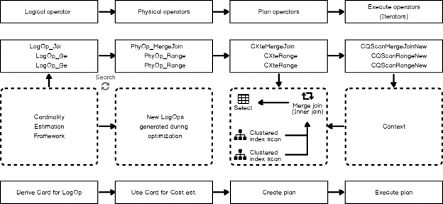
Below you may see the picture of the general plan-building process in SQL Server from the moment when a server receives a query till the storage engine is ready to retrieve the data. Take a quick look first, and next I’ll provide explanations.
There are a lot of nuances and sub-steps left behind this illustration, but they are not important here.
From the cardinality estimation prospection the process consists of the four main steps:
- Derive cardinality for the logical operators
- Use cardinality to cost the physical operators
- Pick the most cheap physical operators and build a compiled plan
- Convert a compiled plan to an executable plan
Now, let’s talk about each step of this process in more details.
Logical Operators Tree
The process begins when the query is first sent to a server. When it is received and read from the TDS protocol, the Parser component comes in. It validates text and parses it into a query tree of logical operators (the other actions are also done on that stage like binding, view or computed columns expansion and so on). You may see the tree as the first green block in the picture.
Next, this tree is simplified (also a lot of work is done here, but not relevant to the post’s topic and abandoned). After that, the first, initial cardinality estimation occurs. It should be done very early to determine the initial join order, that order might be next modified during the query optimization.
You may observe this tree using undocumented TF 8606, to add some details about cardinality estimation to that output this TF might be combined with another undocumented flag TF 8612. It is interesting to include the TF 2372, that outputs some optimization stage memory info and may be used to view some details about the process. We also need TF 3604 to direct output to console.
Let’s perform a simple query in the “opt” database, using these flags:
|
1 2 3 4 5 6 7 8 9 10 11 12 13 14 15 |
use opt; go set showplan_xml on go select * from t1 join t2 on t1.a = t2.b option ( querytraceon 3604, -- Output to console querytraceon 2372, -- Optimization stage memory info querytraceon 8606, -- Logical operators trees querytraceon 8612 -- Add aditional cardinality info ) go set showplan_xml off go |
Now, if you switch to the Message tab in SQL Server Management Studio, you may observe various trees of logical operators. Each tree representation in this diagnostic output reflects the result of the particular plan constructing phase. I’ve described each of them a few years ago in my Russian blog and hope there will be time to do the same in this blog, however not now, because it is not relevant to the topic. If you are interested, you may look through my presentation from SQL Saturday 178, to have an idea what’s going on.
Here, our focus is on cardinality estimation and we are interested in two outputs Simplified Tree (the tree after various simplifications, e.g. contradiction detection or redundancy removing) and Join-collapsed Tree (the tree after initial join reordering and removing unnecessary joins).
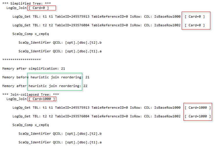
You may notice that Simplified Tree has cardinality equals zero ([Card = 0]), and Join-collapsed tree already has cardinality set to 1000 ([Card = 1000]). Between the two moments, when those trees were output the cardinality estimation process occured.
It should be done before join reordering and it makes sense, because the optimizer may apply reordering heuristics only after it knows what is the expected cardinality and what join order is expected to be better. Later, during the optimization, the initial join order might be changed using various exploration rules, but the more Joins there are, the less percent of changes of the initial order is expected.
This step is depicted as the first, the green one, in the picture above.
- LogOp_Get – stands for the logical operation get a table
- LogOp_Join – stands for the logical operation inner join
- ScaOp_Comp x_cmpEq – stands for scalar operator compare equal, because we have an equality in the join ON clause
- ScaOp_Identifier – stands for the column identifier because we joined on two columns
Physical Operators Tree
Next goes the optimization itself. A lot of alternatives are explored, among them are physical implementations of the logical operators (e.g. Logical inner join to Physical inner merge join), new logical operators, that are equivalent to the one we have so far (e.g. A join B to B join A), or completely new logical operators. You may see this tree as the red block in the picture.
On that stage cardinality estimations are also present, if the new logical alternative appears – it should be estimated. It is also very important part, if something goes wrong here all the next optimization process might be useless.
After that server has a Physical Operators tree that was chosen among the others based on a cost. Cost is assigned only to physical operators. It’s also worth saying, that there are a lot of techniques to avoid exploring high cost alternatives or spending a lot of time exploring all the possible plans. You may have heard of pruning, time out, optimization stages and so on.
When this step is completed, a server has a tree of physical operators. We may observe it in the diagnostic output, if we enable TF 8607, similar as we did before for the logical operators tree.
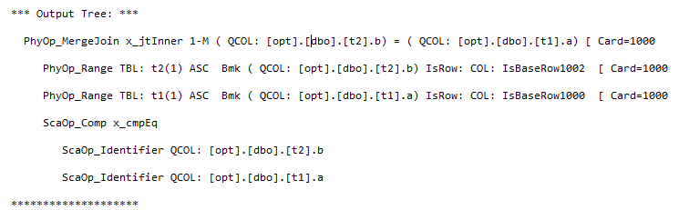
- PhyOp_MergeJoin x_jtInner 1-M – stands for the physical operator of the one-to-many inner merge join
- PhyOp_Range – stands for the physical data access operator
That tree is not the query plan yet. Next comes the rewrite process, that, for example, combines together filters and scan into scan with residual predicate and does some other useful rewrites.
Plan Operators Tree
A plan operator tree, is a structure that we used to call a Compiled Plan and what is saved internally to a plan cache if needed. The other names of this structure are: Query Plan, Execution Plan either Estimated or Actual.
When we demand an execution plan, the internal methods of the plan tree nodes are called and return an XML output. That might be interpreted later by the client (SQL Server Management Studio, for example) and show us a graphical view.
A tale of two different plans
A small interesting note about the differences between an Estimated Execution Plan and an Actual Execution Plan. In some sources, I saw them treated like separate objects, because they may be different. Well, yes, they may be different, however, they are both Compiled Plans.
Consider the following example.
|
1 2 3 4 5 6 7 8 9 10 11 12 13 14 15 16 17 18 |
use opt; go -- Get the Estimated Plan set showplan_xml on go declare @a int = 0; select *, case when @a = 1 then (select top(1) b from t2) end from t1 option(recompile); go set showplan_xml off go -- Get the Actual Plan set statistics xml on go declare @a int = 0; select *, case when @a = 1 then (select top(1) b from t2) end from t1 option(recompile); go set statistics xml off go |
The plans would be different:
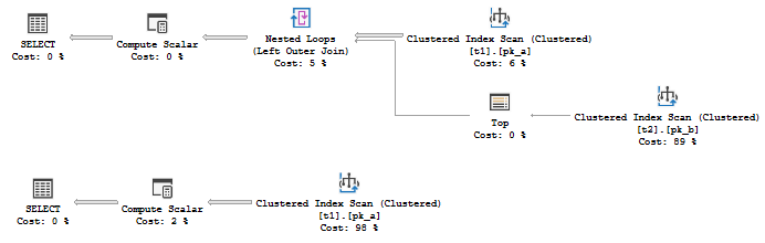
You see, that the second (the Actual one) doesn’t access table t2 at all!
This behavior makes people think, that these are two steps of the one process, and that at first server gets the estimated plan and then it gets the actual plan, two different types of plans. If that was true, that would mean that optimization should be done twice!
If we collect plans with extended events query_post_compilation_showplan and query_post_execution_showplan for the second execution – we will see, that post compilation plan (without any runtime information) has the same shape as the post execution plan and no t2 access.
The difference between the two plans above appears because of a so called Parameter Embedding Optimization. When option recompile is used at the statement level some kind of a deferred compilation is used. Then, when the execution begins, statements in the batch or module are executed one by one until the deferred recompilation statement is achieved. At that moment all the local variables are known and might be embedded into the query as a run-time constants, with this new constants the recompilation occurs.
You may think of the recompiling query as if @a was replaced by its run-time value 0:
|
1 |
select *, case when 0 = 1 then (select top(1) b from t2) end from t1 option(recompile); |
Obviously, condition 0 = 1 could not ever be true, and it is safely removed at the simplification phase. This optimization may be also applied in the where clause, order by clause, join on clause etc.
It is interesting to note, that a plan with an option recompile is cached together with the whole batch plan. That is another proof that there is no special Estimated and Actual plans.
Look at the following example. There is a batch containing three statements, the first one is a declare, the second one is a Join without any recompilation, and the third is a statement with an option recompile.
Let’s demand estimated plan, then execute it and demand estimated plan again.
|
1 2 3 4 5 6 7 8 9 10 11 12 13 14 15 16 17 18 19 20 21 22 23 24 25 26 |
dbcc freeproccache; go --Demand estimted plan: first time set showplan_xml on go declare @a int = 0; select * from t1 join t2 on t1.a = t2.b; --Statement to be cached select *, case when @a = 1 then (select top(1) b from t2) end from t1 option(recompile); --Statement to be recompiled go set showplan_xml off go -- Execute go declare @a int = 0; select * from t1 join t2 on t1.a = t2.b; --Statement to be cached select *, case when @a = 1 then (select top(1) b from t2) end from t1 option(recompile); --Statement to be recompiled go --Demand estimted plan: second time set showplan_xml on go declare @a int = 0; select * from t1 join t2 on t1.a = t2.b; --Statement to be cached select *, case when @a = 1 then (select top(1) b from t2) end from t1 option(recompile); --Statement to be recompiled go set showplan_xml off go |
(Note, that a batch should be the same every time, that’s why I put the comment Execute in a separate batch, splitting with GO)
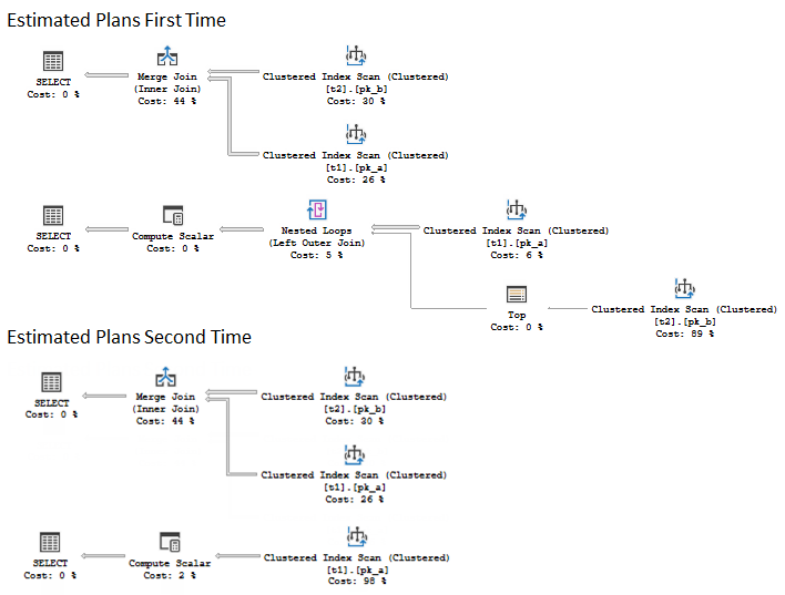
Surprisingly, we may see that the pair of the estimated execution plans, that was demanded after the execution has the different plan for the second query. It is the compiled plan, that was cached after recompilation during the execution. Interesting to note, that if you inspect the property of the SELECT language element (the green icon) in the second plan, you will find the property “RetrievedFromCache” set to “false”, however, if you inspect the plan cache:
|
1 2 3 4 5 6 7 8 9 10 |
select qp.query_plan, st.[text] from sys.dm_exec_cached_plans cp cross apply sys.dm_exec_query_plan(cp.plan_handle) qp cross apply sys.dm_exec_sql_text(cp.plan_handle) st where st.[text] like '%Statement to be cached%' and st.[text] not like '%dm_exec_cached_plans%' |
Both plans will be returned.
I think that is enough to demonstrate that there is no two separate different plans like Estimated and Actual. These terms are a little bit confusing (implying the difference, according to the title), but very widespread. In the new Extended Events mechanism, the plans are called in a more correct way: post compilation, pre execution, post execution. I simply call it a compiled plan. An actual plan is an XML or text representation of a compiled plan with additional run-time info.
That’s what a Compiled Plan is, but still, it is still not what would make the actual iterations over rows.
Executable Operators Tree (Iterators Tree)
When a plan is compiled and should be next executed, server turns a Compiled Plan into an Executable Plan (don’t mix it with an Actulal Execution Plan), also known as an Execution Context.
There might be one compiled plan, but several executable plans. That makes sense as there might be multiple users who want to execute the same query. Also, the query may have variables and each user may provide specific values for them. That should be considered in the execution, and so, the execution context is built.
Also, each execution context might track the actual number of rows or any other execution specific information and combine it with a compiled plan, and so we get back what is called an Actual Plan if we demand.
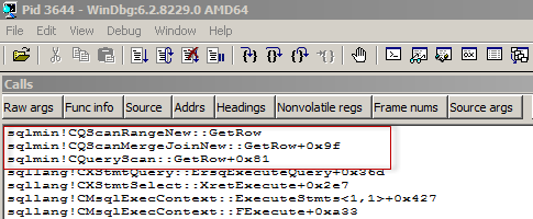
An Executable Plan is represented as the last, purple blocks in the picture. There are no TFs or any other ways to view it directly (or I don’t know them), the only way I know, is to use a debugger with debug symbols.
I’ll provide a screenshot how it looks like in WinDbg for the illustration.
Back to Cardinality Estimation
We observed the main optimization process, and learned that the Cardinality Estimation process is used during the very first step and is used next during the second step of a query optimization. If these initial steps produce inaccurate estimates all the next steps and the query execution may be very inefficient due to the inefficient plan. That is why cardinality estimation is so important mechanism in a query optimization process.
The last thing I’d like to mention in that post is that cardinality estimation is done over logical operators only, as we saw. If we think about it – it makes sense. For example, if we join table using Loop Join and get 10 rows, but with Hash Join get 11 rows – obviously, there is something wrong with the join algorithm. It should not work this way.
Let’s create an index and look at the example.
|
1 2 3 4 5 6 7 8 9 10 |
create index ix_b on t1(b); go set showplan_xml on go select t1.b, t2.b from t1 join t2 on t2.b = t1.b join t3 on t3.c = t2.b where t1.b < 300 option(loop join) select t1.b, t2.b from t1 join t2 on t2.b = t1.b join t3 on t3.c = t2.b where t1.b < 300 option(merge join) go set showplan_xml off go drop index t1.ix_b; |
The same query but with different hints for the join algorithm. Every single Join has the same estimates, according to the plans.
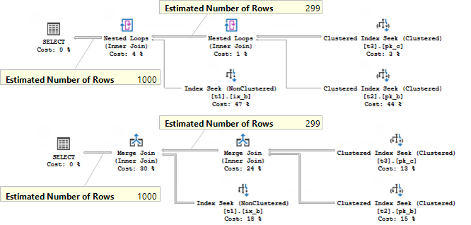
But it is worth to remember that the estimation is dependent of the new logical groups, that may appear during the optimization. If we add some grouping using distinct into this artificial example, we will see, that now estimates of the join types are different.
|
1 2 3 4 5 6 7 8 9 10 |
create index ix_b on t1(b); go set showplan_xml on go select distinct t1.b, t2.b from t1 join t2 on t2.b = t1.b join t3 on t3.c = t2.b where t1.b < 300 option(loop join) select distinct t1.b, t2.b from t1 join t2 on t2.b = t1.b join t3 on t3.c = t2.b where t1.b < 300 option(merge join) go set showplan_xml off go drop index t1.ix_b; |
You may see that now estimates for the Loops Join and Merge Join are different.
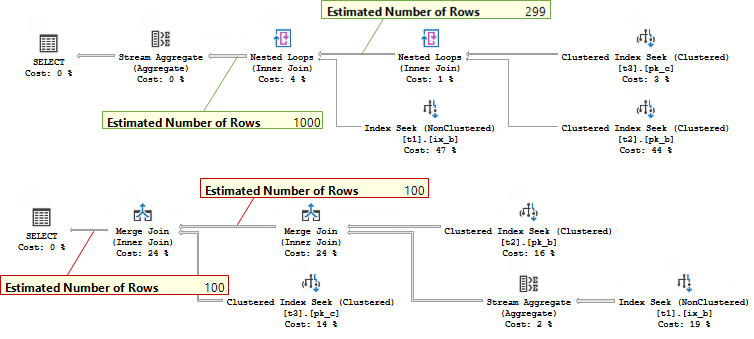
But that is not because the different physical join types are estimated differently, but because the join type drove optimizer to choose another plan shape, and it was considered to be cheaper to perform the aggregation before the Join in case of a Merge Join. That changed cardinality input for the Join and lead to different estimate.
That’s all for today, in the next post we’ll talk about the cardinality estimation main concepts.
Table of Contents
References
- Cardinality Estimation (SQL Server)
- SQL Server 2014’s new cardinality estimator (Part 1)
- The New and Improved Cardinality Estimator in SQL Server 2014

Currently he works as a database developer lead, responsible for the development of production databases in a media research company. He is also an occasional speaker at various community events and tech conferences. His favorite topic to present is about the Query Processor and anything related to it. Dmitry is a Microsoft MVP for Data Platform since 2014.
View all posts by Dmitry Piliugin
- SQL Server 2017: Adaptive Join Internals - April 30, 2018
- SQL Server 2017: How to Get a Parallel Plan - April 28, 2018
- SQL Server 2017: Statistics to Compile a Query Plan - April 28, 2018