
In this post, we are going to take a deeper look at the cardinality estimation process. We will use SQL Server 2014, the main concepts might also be applied to the earlier versions, however, the process details are different.
Calculators
The algorithms responsible for performing the cardinality estimation in SQL Server 2014 are implemented in the classes called Calculators.
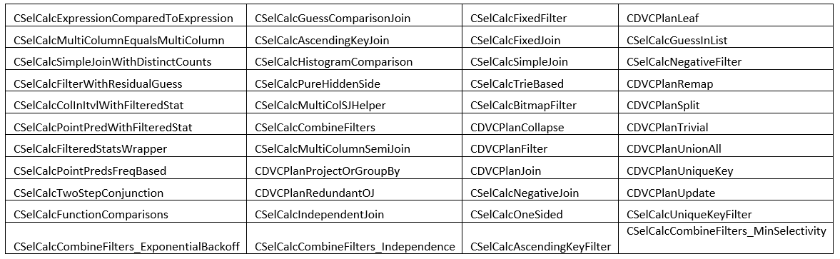
CSelCalc – Class Selectivity Calculator.
CDVC – Class Distinct Value Calculator.
To be more specific, these classes might not contain the one estimation algorithm, rather they join together a set of specific algorithms and drive them. For example calculator CSelCalcExpressionComparedToExpression may estimate join cardinality using join columns histograms in a different ways, depending on the model variation, and the specific estimation algorithms are implemented in the different classes, used by this calculator.
I mentioned a model variation – this is another new concept in the new cardinality estimation framework. One of the goals of implementing the new cardinality estimation mechanism was to achieve more flexibility and control over the estimation process. Different workload types demand different approaches to the estimation and there are some special cases when two approaches may contradict each other. Model variations are based on a mechanism of pluggable heuristics and may be used in special cases.
SQL Server 2014 has additional diagnostic mechanisms which allow us to take a closer look at how the estimation process works. These are trace flag 2363 and extended event query_optimizer_cardinality_estimation. They might be used together to get the maximum of the estimation process details.
The Estimation Process
Let’s consider a simple example of a query, in database “opt” , that selects from the table and filter rows.
|
1 2 3 4 5 6 7 8 |
use opt; go set showplan_xml on go select * from t1 where b = 100 option(querytraceon 9130) go set showplan_xml off go |
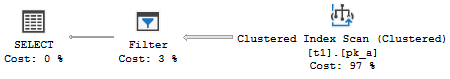
Note: Normally, the optimizer would join together a filter and a scan operator on the phase when the Physical Operators Tree is converted to the Plan Operators Tree (this process is known as Post Optimization Rewrite), to avoid a separate Filter plan operator and reduce the cost of passing rows between Filter and Scan operator. To prevent this, for demonstration purposes, I use trace flag 9130, that disables this particular rewrite.
This query has the following simple plan:
Let’s use the undocumented TF 2363, mentioned above, to view diagnostic output. We also use TF 8606, described in the previous post, to view logical operators tree with TF 8612 to add cardinality info. TF 3604 is also necessary to direct output to console.
|
1 2 3 4 5 6 |
set showplan_xml on go select * from t1 where b = 100 option(querytraceon 9130, querytraceon 8606, querytraceon 8612, querytraceon 2363, querytraceon 3604) go set showplan_xml off go |
If we switch to the message tab, we’ll see the following output:
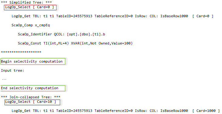
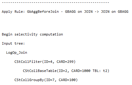
Between the two trees of the logical operators, there is some additional output that starts with the phrase “Begin selectivity computation” and ends with “End selectivity computation”. I copied this output to the image below and painted it, to give some explanations.
The TF Output:
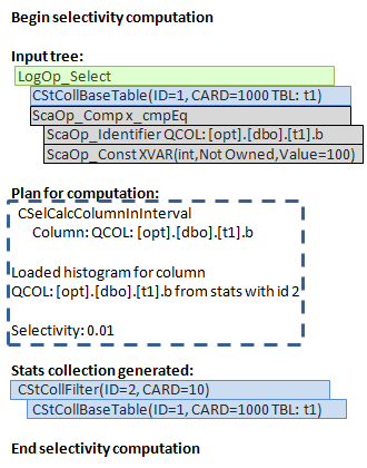
The Process:
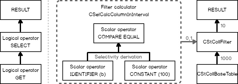
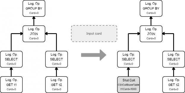
The process starts with the input tree of logical operators. For that simple case there are only two of them:
- LogOp_Get – gets the table
- LogOp_Select – selects from the table, this is a relational select, that means “select from set”, i.e. filtering
- Scalar operators – determine the comparison condition, here we have an equality check for a column and a constant
The tree is depicted on the left of the second picture. The cardinality calculation goes bottom-up, starting from the lowest operator (or the up-right if we look at the graphical plan). In the diagnostic output, we see that a base table statistics collection was loaded for the lowest logical operator “get table”.
Next, the filter selectivity should be computed. For that purpose, the plan for selectivity computation is selected, in our case, this would be the calculator – CSelCalcColumnInInterval. The one may ask, why “interval”, if there is an equality comparison. The answer is, that our column is not unique and so several rows are possible. If it had a unique constraint or index the calculator would be CSelCalcUniqueKeyFilter.
The calculator computes the selectivity using input statistics from the operator get (the output even tells us what histogram was loaded), and a set of algorithms, that represents this type of calculator and are based on the mathematical model, discussed in the previous post. The computed selectivity is 0.01.
This selectivity is multiplied by the input cardinality of 1000 rows and we have an estimate: 1000*0.01 = 10 rows. Perfect!
The next step, takes this cardinality, modifies density and histogram according to it, and generates a new statistics collection – filter statistics collection. If we had a more complex plan, this statistics collection might be used as an input statistics for the next logical operator, which is higher than Filter, and so on. This process goes from bottom to top, until all the tree nodes will have an estimate.
More complex example
The query below joins two tables, filters and groups data for the distinct purposes.
|
1 2 3 4 5 6 7 8 9 10 11 12 13 |
set showplan_xml on go select distinct t1.b, t2.b from t1 join t2 on t2.b = t1.b where t1.b < 300 option(recompile, merge join , querytraceon 3604 -- <-- Output to Console , querytraceon 8606 -- <-- Show LogOp Trees , querytraceon 8619 -- <-- Show Applied Transformation Rules , querytraceon 8612 -- <-- Add Extra Info to the Trees Output , querytraceon 2363 -- <-- (2014, new:) TF Selectivity ); go set showplan_xml off go |
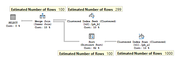
It has the following plan:
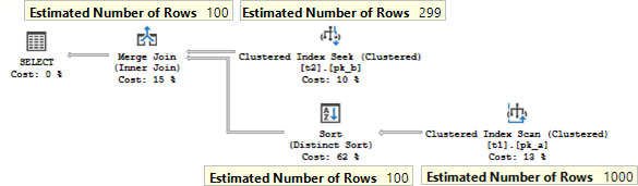
A few notes about this plan.
The DISTINCT clause is used in the query, that means only unique pairs of values t1.b and t2.b should be returned. To satisfy this, the server uses grouping by means of the operator Stream Aggregate. What is worth noting, that one of the grouping columns – column t2. b has a primary key defined, therefore, is unique, because of that, the server may not group by that column and leave only t1.b for the aggregation. That means that the aggregation could be safely done before the join, to reduce the number of joining rows.
We filter on the t1.b column and join on it also, so the filter could be applied to t2.b column also. The filter operator itself is not present in the plan as a separate plan operator, it is combined with a seek and scan.
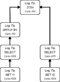
The logical operator tree for that query looks like this:
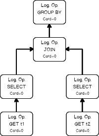
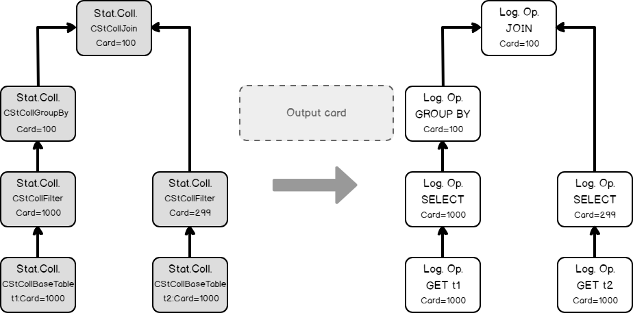
Let’s now watch, how goes the estimation process. I’ll not provide a TF diagnostic output here, because it is too verbose, rather, I’ll convert it into a graphical form, the series of pictures.
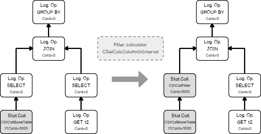
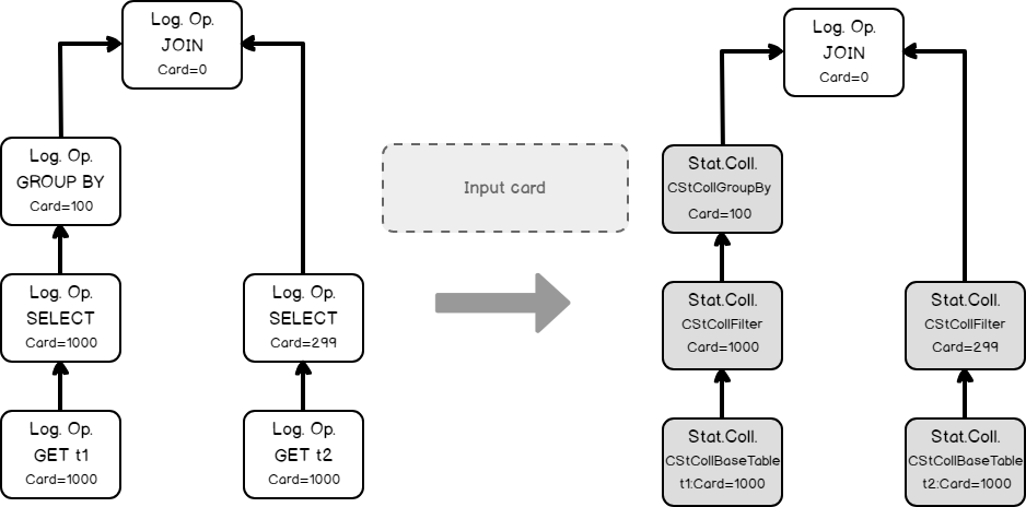
The input tree of the logical operators, loading statistics collection of the base table.

Estimating the filtering condition for column t1, as we saw in the previous simple example, and creating the new statistics collection.
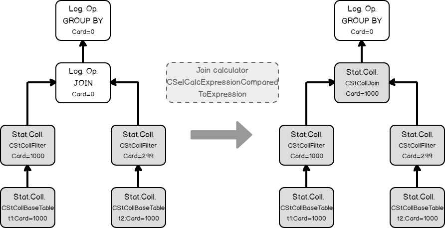
- Doing the same thing with table t2, loading base statistics.
Estimating the filtering condition for t2.b (remember the filter was propagated, from t1.b because of the join equality comparison on the same column).
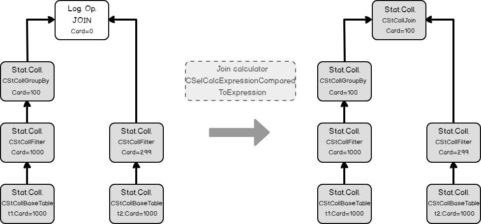
Now we have all necessary input to estimate the join cardinality. Using filters statistics collection and the join calculator CSelCalcExpressionComparedToExpression to estimate the join cardinality. Note: in fact, the join may use base table statistics and combine it with a filter selectivity – this called Based Containment Assumption, but we will not delve into it here, because it’s worth a separate blog post.
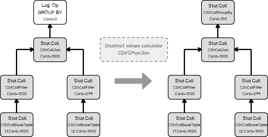
Finally, using the join statistics collection we are ready to calculate the cardinality of a grouping operation.
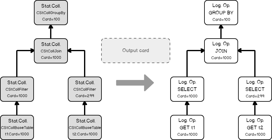
Now we may set calculated cardinalities to the logical operator tree accordingly.
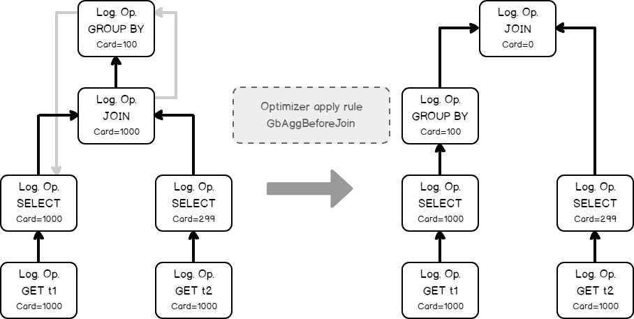
At that moment we have the initial tree with set cardinalities. But as we remember from the previous post, the cardinality estimation occurs during the optimization process also, when the new logical group appears. This is the case. The optimizer decides that it will be beneficial to perform grouping before the join, to lower the number of joining rows. It applies the transformation rule, that generates the new alternative logical group and switches the Join and the Grouping (Group By Aggregate Before Join)..
The new group should also be estimated, because it’s cardinality is unknown.
The optimizer once again uses the input statistics of the child nodes.
Using the same calculator CSelCalcExpressionComparedToExpression, the optimizer estimates the new logical group.
Now again, all the cardinalities are known.
Later the logical Get and logical FIlter would be implemented as the Seek with a predicate and the Scan with a residual predicate, then the logical Join would be transformed to the physical Merge join and the group operator into the physical Stream Aggregate.


That’s how it works!
I’d like you to take out of this part one very important thing, that might be applied in practice. As you saw, the estimation goes from bottom to top, using child node statistics as an input to estimate a current node. If the estimation error appears at some step, it is propagated further, to the next operators. That’s why, when you try to struggle with inaccurate cardinality estimates, try to find the bottom most inaccurate estimate. Very likely it skewed all the next estimates. Don’t struggle with the top most inaccuracy, because this inaccuracy might be induced by the previous operators.
For the truth, I should say, that sometimes there are curious cases, when the two incorrect estimates annihilate each other negative impact, and the plan is fine. If you eliminate one of them, the fragile balance is ruined and the plan becomes a problem. By the way, that is one of the reasons, why Microsoft was very conservative to introduce new changes to the cardinality estimation and left them “off” by default and demand a trace flag to use it.
In the next post we’ll see how the “old” cardinality estimation behavior may be used in SQL Server 2014.
Table of Contents
References
- Cardinality Estimation (SQL Server)
- Testing cardinality estimation models in SQL server
- What’s New (Database Engine, SQL Server 2014)

Currently he works as a database developer lead, responsible for the development of production databases in a media research company. He is also an occasional speaker at various community events and tech conferences. His favorite topic to present is about the Query Processor and anything related to it. Dmitry is a Microsoft MVP for Data Platform since 2014.
View all posts by Dmitry Piliugin
- SQL Server 2017: Adaptive Join Internals - April 30, 2018
- SQL Server 2017: How to Get a Parallel Plan - April 28, 2018
- SQL Server 2017: Statistics to Compile a Query Plan - April 28, 2018