
This article is the second part of the Nested Loop Join Series. In the first part, Introduction of Nested Loop Join, we gave a brief introduction to Native, Indexed and Temporary Index Nested Loop Joins along with CPU cost details.
The second part shows how parallelism is implemented in the Nested Loop Join, a brief introduction about a few Outer Row Optimizations and interesting concepts about the inner side of the Nested Loop Join.
Parallel Nested Loop Join
In this section we will concentrate on parallel processing in the Nested Loop Join. Before we start this article, I would like to explain a bit about the Parallel Page Supplier, because it helps in understanding the Nested Loop Join as a whole.
Whenever parallel scan/seek is initiated on the table, a storage engine feature called the Parallel Page Supplier performs its task of distributing a set of pages to the available threads on the basis of the demand based schema.
When a thread finishes with its assigned set of pages, it requests the next set of pages from the parallel page supplier. The demand based schema balances the load efficiently, if one thread runs slower than the other threads for any reason. For example, if a thread is busy doing some other processing, then that thread simply requests fewer pages while the other threads pick up the extra work.
For a better understanding about Parallel Nested Loop Join, we will insert more rows to the DBO.T1 table and create a new NL_Parallel table. The script for this can be found below.
|
1 2 3 4 5 6 7 8 9 10 11 12 13 |
Insert into [DBO].[T1] Select Primarykey +100000 ,Primarykey +100000 , Primarykey +100000 , SomeData from [DBO].[T1] Create Table NL_Parallel (PrimaryKey INT NOT NULL CONSTRAINT PK_PrimaryKey PRIMARY KEY , KeyCol varchar(50) , SearchCol int , SomeData char(8000) ) Insert INTO NL_Parallel SELECT * FROM T1 WHERE Primarykey < 50001 GO |
In the below query, we are controlling the query to choose the specific execution plan by using Option clause, so that we can get the identical execution plan. But if in case you are unable to get it then please run the script of statistics copy of the above tables on your system from below the article.
|
1 2 3 4 5 6 7 8 9 10 11 12 13 14 15 |
SELECT * FROM NL_Parallel OT1 JOIN T1 ot2 ON ot1.Keycol = ot2.Keycol WHERE OT1.SearchCol IN (101,102,103,104,105,106,107,108,109,110, 111,112) OPTION (LOOP JOIN -- Choose only nested loop join as physical join type ,RECOMPILE -- Compile and create execution plan again ,Querytraceon 8649 -- Undocumented: Force query optimizer to choose a parallel plan ,Force Order -- to match the logical expressed query to physical query plan ,MaxDop 4 -- Run with 4 logical processors ) |
Let us first look at the estimated execution plan.
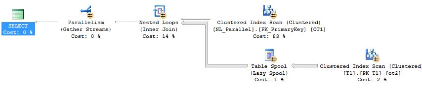
The unexpected Table Spool (if you want to learn strictly about the parallel execution plan in the nested loop join you can skip this subsection)
The major features of this execution plan is the Table Spool (Lazy spool, not to be confused with the index spool). A Table Spool (Lazy spool) is a part of the optimization process. The Query Processor creates a hidden temporary table in the Tempdb database, which inserts the rows in the Table Spool only when requested by the parent iterator, and it is a non blocking operator. But is it required here?
To give a non-theoretical answer, we will execute two versions of the query one with Table Spool and another without it and we will investigate the results.
|
1 2 3 4 5 6 7 8 9 10 11 12 13 14 15 16 17 18 19 20 21 22 23 24 25 26 27 28 29 30 31 32 33 |
SET STATISTICS TIME,IO ON SELECT * FROM NL_Parallel OT1 JOIN T1 ot2 ON ot1.Keycol = ot2.Keycol WHERE OT1.SearchCol IN (101,102,103,104,105,106,107,108,109,110, 111,112) OPTION (LOOP JOIN -- Choose only nested loop join as physical join type ,RECOMPILE -- Compile and create execution plan again ,Querytraceon 8649 -- Force query optimizer to choose a parallel plan ,Force Order -- to match the logical expressed query to physical query plan ,MaxDop 4 -- Run with 4 logical processors ) Print '2nd Query started' SELECT * FROM NL_Parallel OT1 JOIN T1 ot2 ON ot1.Keycol = ot2.Keycol WHERE OT1.SearchCol IN (101,102,103,104,105,106,107,108,109,110, 111,112) OPTION (LOOP JOIN -- Choose only nested loop join as physical join type ,RECOMPILE -- Compile and create execution plan again ,Querytraceon 8649 -- Force query optimizer to choose a parallel plan ,Querytraceon 8690 --disable spooling in query plan ,Force Order -- to match the logical expressed query to physical query plan ,MaxDop 4 -- Run with 4 logical processors ) |

In the second query we used trace flag 8690 which is an undocumented trace flag and is not recommended at all in the production server. Statistics IO and Statistics Time information is also gathered for better understanding of the execution related metrics.
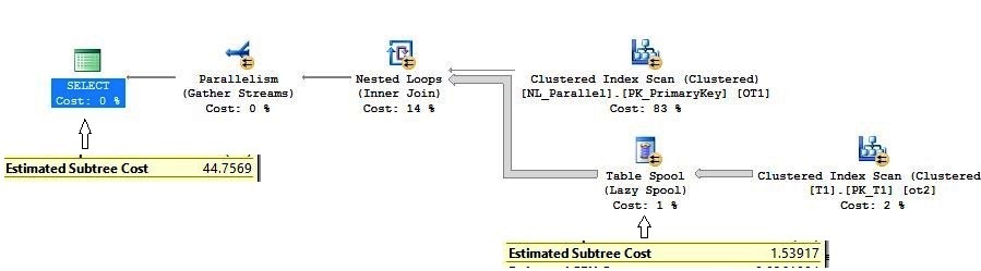
Estimates of the query are pretty accurate, and the subtree cost of the top and bottom query is 44.7569 and 46.8445 respectively. If observed closely we can see that the difference came because of inner side of nested loop join.
On the top query, Table Spool’s subtree cost is estimated 1.53917 units.
At bottom of the execution plan, on the inner side of nested loop join it is 3.62677.
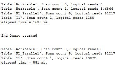
Now let us look at the message tab, for top query, there are two Worktables (Worktables are internal tables that hold intermediate results). One of them represents the Table Spool directly, on my system for the top query, 546866 additional logical reads are reported and it executes in 1630 ms, whereas for the bottom query there is no additional IO for the worktable and the query is executed in 551 ms.
In my opinion, for the above scenario, there is no reason to have a Table Spool. The Table Spool is just additional overhead, since there is no filter predicate for the inner table DBO.T1. If there was any filter, DBO.T1 would have passed only some pages to Table Spool and further execution would have occurred from the newly created Table Spool. But in the above execution plan, it is passing the whole table to Table Spool, which would lead some additional IOs, TempDB Overhead and some other Table Spool related overheads.
SQL Server uses cost based optimization to choose the final execution plan for the query, and in the optimizer reasoning, using a Table Spool would be slightly better than non-Table Spool version of the query. The Query Optimizer uses some assumptions which influence the cost of the execution plan. One of the major assumption which influence the plan choice is that every query starts with cold cache, also known as cold cache assumptions. So, it is possible that in the last execution cache was warm, hence try to execute it this time with the cold cache.
COLD CACHE TEST
In this test we will run both the above queries, but this time with cold cache. To clean the buffer cache we will use the DBCC DropCleanBuffers command, which is not recommended on the production server.
|
1 2 3 4 5 6 7 8 9 10 11 12 13 14 15 16 17 18 19 20 21 22 23 24 25 26 27 28 29 30 31 32 33 34 35 36 37 38 39 |
CHECKPOINT; Dbcc Dropcleanbuffers; SELECT * FROM NL_Parallel OT1 JOIN T1 ot2 ON ot1.Keycol = ot2.Keycol WHERE OT1.SearchCol IN (101,102,103,104,105,106,107,108,109,110, 111,112) OPTION (LOOP JOIN -- Choose only nested loop join as physical join type ,RECOMPILE -- Compile and create execution plan again ,Querytraceon 8649 -- Force query optimizer to choose a parallel plan ,Querytraceon 8690 --disable spooling in query plan ,Force Order -- to match the logical expressed query to physical query plan ,MaxDop 4 -- Run with 4 logical processors ) Print '2nd Query started' CHECKPOINT; Dbcc Dropcleanbuffers; SELECT * FROM NL_Parallel OT1 JOIN T1 ot2 ON ot1.Keycol = ot2.Keycol WHERE OT1.SearchCol IN (101,102,103,104,105,106,107,108,109,110, 111,112) OPTION (LOOP JOIN -- Choose only nested loop join as physical join type ,RECOMPILE -- Compile and create execution plan again ,Querytraceon 8649 -- Force query optimizer to choose a parallel plan ,Force Order -- to match the logical expressed query to physical query plan ,MaxDop 4 -- Run with 4 logical processors ) |
To conclude the test, I ran both the scripts 10 times. The Top query which is without a spool ran in 46.86 seconds while the bottom query which has a Table Spool ran in 47.01 seconds. However, we should not trust the close numbers because when the query is running, the machine’s state matters. Even in an idle system, some background processes run, which consumes resources.
So, this justifies the execution plan costs to a limit, but still there is some additional Tempdb consumption, which is related to the Table Spool.
However, this topic was not the main thrust of this article so, now, we will segue back to a discussion of parallel nested loop joins.
Parallel Nested Loop Join
To remove complexity from the execution plan, we are removing the Table Spool using the trace flag 8690. Again, remember that this is an undocumented trace flag and is not recommended for use on a production server.
|
1 2 3 4 5 6 7 8 9 10 11 12 13 14 15 16 |
SELECT * FROM NL_Parallel OT1 JOIN T1 ot2 ON ot1.Keycol = ot2.Keycol WHERE OT1.SearchCol IN (101,102,103,104,105,106,107,108,109,110, 111,112) OPTION (LOOP JOIN -- Choose only nested loop join as physical join type ,RECOMPILE -- Compile and create execution plan again ,Querytraceon 8649 -- Force query optimizer to choose a parallel plan ,Querytraceon 8690 --disable spooling in query plan ,Force Order -- to match the logical expressed query to physical query plan ,MaxDop 4 -- Run with 4 logical processors ) |
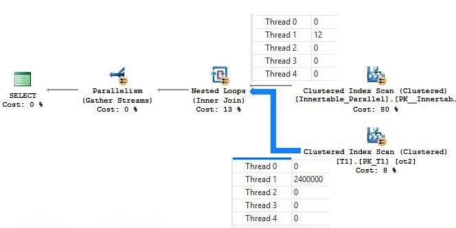
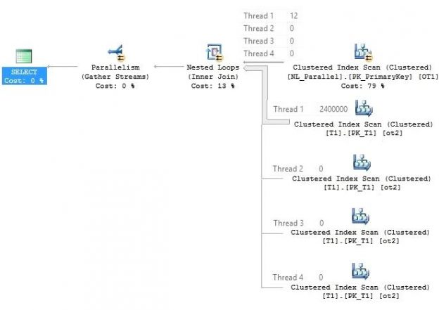
Have a look at the above query plan’s outer table. There exists a parallel scan, thus parallel page supplier (parallel page supplier is not a part of the relational engine so it cannot be seen in the execution plan) distributes a bunch of rows to all the threads. Then the filter is applied on all the active threads. All the rows that satisfy the filter predicate are in the thread 1 (Depends on the timings and data structure of the table, if you keep running the query you might see the rows in different threads).
The inner side of the parallel Nested Loop Join executes as per the outer side of the thread’s execution. To have a better understanding we have elaborated the inner side of an execution plan.

As we can see in the outer table, only thread 1 has all the filtered rows, other threads do not have any rows at all. Thus, on the inner side of the loop join only thread 1 will take part in this activity while the rest of the threads won’t able to take part in this.
Let us change the constant literal values for the above query and see the execution plan.
|
1 2 3 4 5 6 7 8 9 10 11 12 13 14 15 16 |
SELECT * FROM NL_Parallel OT1 JOIN T1 ot2 ON ot1.Keycol = ot2.Keycol WHERE OT1.SearchCol IN (101,102,103,504,505,506 ,1007,1008 ,1009,2010 , 2011,2012) OPTION (LOOP JOIN -- Choose only nested loop join as physical join type ,RECOMPILE -- Compile and create execution plan again ,Querytraceon 8649 -- Force query optimizer to choose a parallel plan ,Querytraceon 8690 --Disable spooling in query plan ,Force Order -- To match the logical expressed query to physical query plan ,MaxDop 4 -- Run with 4 logical processors ) |
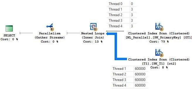
Now look at the above execution plan on the NL_Parallel table. All four threads have equal amount of rows and, because of that, the inner side of execution processed is parallel. This execution plan is slightly better than the above execution plan, as it uses the Parallelism evenly in the inner table.
Prior to SQL Server 2008, the Nested Loop Join has a problem in processing the inner side, in a similar way as it brought rows from the outer table scan/seek. Usually this is not a problem when a lot of rows are encountered in the outer table, but it is not optimal in situations where when the rows are uneven in the threads. But now, in SQL Server 2008 and later versions, the Query Optimizer can add the exchange iterator to distribute outer tables’s rows evenly, so that the inner side can take full advantage of the parallelism. This process is called Few Outer Rows Optimization.
Alert readers might be thinking that if a Few Outer Rows Optimization was available for SQL Server 2008 and above versions, then why this was not observed on the above test machine.
There are actually some cases where Few Outer Rows Optimization does not start and the above case was one such example. NL_Parallel table has LOB data type (somedata char(8000)), therefore let us change the data size and then examine the query plan again.
|
1 2 3 4 5 6 7 8 9 10 11 12 13 14 15 16 17 18 19 |
ALTER TABLE NL_Parallel ALTER COLUMN SomeData char(20) ALTER TABLE NL_Parallel REBUILD -------------------------------------------------------------------------------------------- SELECT * FROM NL_Parallel OT1 JOIN T1 ot2 ON ot1.Keycol = ot2.Keycol WHERE OT1.SearchCol IN (101,102,103,104,105,106,107,108,109,110, 111,112) OPTION (LOOP JOIN -- Choose only nested loop join as physical join type ,RECOMPILE -- Compile and create execution plan again ,Querytraceon 8649 -- Force query optimizer to choose a parallel plan ,Querytraceon 8690 --disable spooling in query plan ,Force Order -- to match the logical expressed query to physical query plan ,MaxDop 4 -- Run with 4 logical processors ) |
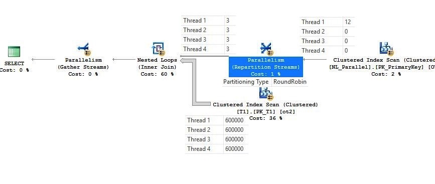
In the above execution plan, at the outer input, it is the additional exchange iterator “round robin” type, which distributes all the rows evenly to all the available threads and because of that all the threads run evenly at the inner side as well. The exchange iterator is not a part of optimization, it is actually post optimization rewrite.
Estimation VS Actual Row count At the Inner Side
Whenever we tune a long running query, we check the execution plan quality by looking at the different aspects of the execution plan, one of them is the estimated and actual row count difference.
If the difference of actual and estimated row count is huge and if it degrades the quality of the plan, we try to optimize that particular portion of the query plan.
But usually the Nested Loop Join’s inner side is an exception, even if the histogram represents the data distribution accurately, the difference between estimated and the actual row count is still observed. To demonstrate that we are using two tables DBO.T1 and DBO.T2 from this series:
|
1 2 3 4 5 6 7 8 9 10 11 |
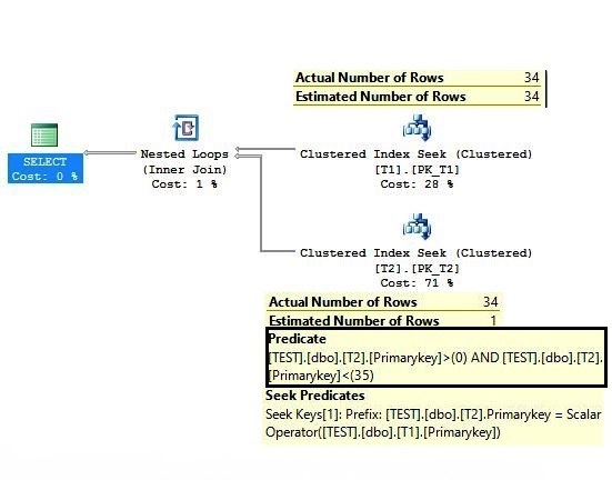
SELECT * FROM DBO.T1 JOIN DBO.T2 ON T1.Primarykey = T2.Primarykey WHERE T1.Primarykey > 0 AND T1.Primarykey < 35 ORDER BY T1.Primarykey OPTION (RECOMPILE) |
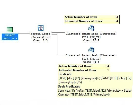
In the above execution plan, the difference of actual and estimated row count at the outer table should be observed. It is found to be perfect. Now take a look into the inner table’s estimation, and we can see the difference. On the inner side the estimated number of rows is 1 and the actual number of rows is 34.
Let us try to debug the inner side, and analyze the origin of this difference? If you look at the query, the JOIN condition and WHERE predicate, both are on the primary key column. Look at the inner side on the DBO.T2 table, the same predicate is also applied, but this is not specified in the query.
Actually, it is a part of the optimization process called Simplification, which we will look in detail in the next section of the article. The question is, why there is the difference of row count on the inner side of query. To find out the estimated number of rows, let us break the above query and apply the predicate directly to DBO.T2 table.
|
1 2 3 4 5 |
SELECT * FROM DBO.T2 WHERE Primarykey > 0 AND Primarykey < 35 |
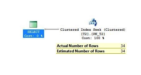
There is no difference between estimated and actual row count values here. So what is the problem with the inner side of nested loop join, why is it misestimated the number of rows, is it buggy?
No, we don’t need to worry about that because for Nested Loop Join’s inner side is calculated as per execution, irrespective of outer table’s rows. Actually, the term used “Estimated number of rows” is misleading here, it should have “Estimated number of rows per execution”.
There is a connect item filed by Hugo Kornelis for this issue, which can be found here.
If the Naive Nested Loop Join is used, then the estimated rows of the inner side would be the table’s cardinality (total estimated number of rows in the table) and if the Index Nested Loop Join is applied and the inner side of index is marked as a unique index (Joining Column(s)), then estimated rows would be 1. But if the inner side of the loop join index is not unique then estimated depends on the cardinality of the joining output, unless row goal applied.
It can be calculated as:
Estimated Output Rows / Inner Table’s Estimated Number of Execution = Inner Table’s Estimated Rows.
Unnecessary Residual Predicates (Only when the JOIN and WHERE column(s) are same)
In this section of the article we see an unusual case, which only occurs with a Nested Loop Join, when the Join and the Where predicates are on the same column(s). We simply use the above query, and explore the case. The query is provided below with execution plan:
|
1 2 3 4 5 6 7 8 9 10 11 |
SELECT * FROM DBO.T1 JOIN DBO.T2 ON T1.Primarykey = T2.Primarykey WHERE T1.Primarykey > 0 AND T1.Primarykey < 35 ORDER BY T1.Primarykey OPTION (RECOMPILE) |
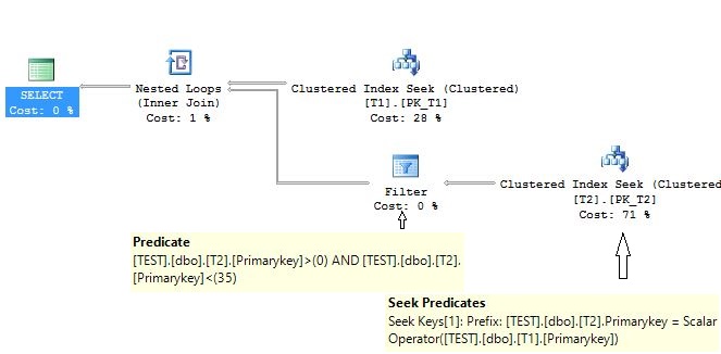
The explanation of the execution is same as above. The part worth noticing is the inner side of Nested Loop Join’s predicate on the DBO.T2 table, which was not a part of the original query.
It is actually an undesired residual predicate, which is just an additional overhead. Because after seeking the row in the Inner side of the Indexed Nested Loop Join, an additional filter is applied during the execution, which is unnecessary in prospect of the above execution.
The residual predicate usually collapses with the child iterator, that is why we can’t see it in the execution plan, but there is an undocumented trace flag 9130 which can be used to see this residual predicate in the query plan. It is not recommended to use this trace flag in production though, as it is undocumented.
|
1 2 3 4 5 6 7 8 9 10 11 |
SELECT * FROM DBO.T1 JOIN DBO.T2 ON T1.Primarykey = T2.Primarykey WHERE T1.Primarykey > 0 AND T1.Primarykey < 35 ORDER BY T1.Primarykey OPTION ( QueryTraceON 9130 ) |
As far as I know this additional predicate cannot be avoided and ideally this residual predicate should not be present here. The question then arises that why is this residual predicate present in the above execution plan?
To understand it, we have to go back to the query optimization stages and look into the process where the query text is translated into the logical tree. To see this process, we will again use some undocumented trace flags 3604 and 8606 which are not recommended to run on the production systems.
|
1 2 3 4 5 6 7 8 9 10 11 |
SELECT * FROM DBO.T1 JOIN DBO.T2 ON T1.Primarykey = T2.Primarykey WHERE T1.Primarykey > 0 AND T1.Primarykey < 35 Order BY T1.Primarykey Option (Querytraceon 3604 , QUERYTRACEON 8606); |
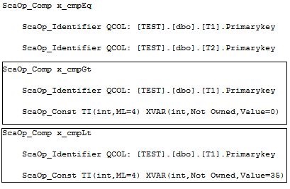
Look at the output of logical tree, we have shortened the output a little bit for better illustration. It is also called an input or converted tree. It is a text conversion of the above query. There is a lot of information in the input tree, but we will focus to the where condition only.
You can see, it is clearly stated that x_cmpGt (Compare greater than) is applied to the T1.primarykey Column with the value of 0. In short, it is implied as T1.Primarykey > 0.
The x_cmpLt (Compare less than) is applied to the T1.primarykey Column with the value of 35. In short it implies as T1.Primarykey < 35.
The simplification is the next stage in the query optimizer pipeline. It tries to rewrite the logical operations around to help this transformation in later stages. It is a good help to the optimizers, sometimes even it stops the optimizer from doing any work from here onwards to save resources in later stages.
In the future, I will write a full length article to explore simplification in more detail. For now, look at the output after simplification phase:
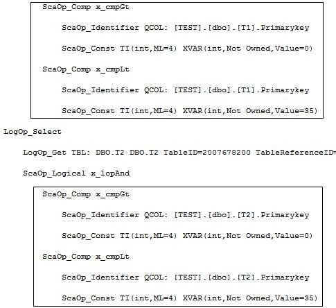
You can clearly see a predicate is applied to the both tables and yes, it is a good decision, because at this stage the Query Optimizer has no idea what physical join will choose after completion of the optimization process. It is a possibility that it might choose the other two physical joins, Merge Join or Hash Match.
If the final selection of join type is Hash or Merge Join, then it is always better to filter the rows as early as possible and pass the least number of rows to the physical join Iterator.
But for the indexed Nested Loop Join there is slight overhead and I assume Microsoft is aware of that situation, but it is ignored as it does not cost much in terms of the execution time.
In this article, we discussed some interesting features about the Nested Loop Join like Parallel Nested Loop Join, Few Outer Row Optimization, Inner side of Nested Loop Join and Residual Predicate.
This series has not ended with this. We will come up shortly with the next article of this series.
I am ending this article with a question. Which physical Join type does not require an additional memory during execution? Please answer in the comment box below.
Download the copy of the statistics.
The previous article in this series
Useful Links
- Parallel processing in SQL Server
- Parallel Page Supplier
- Option Clause (Transact-SQL)
- Table Spool in Execution Plan
- Trace flag 8690
- Statistics IO and Statistics Time
- Worktables
- DBCC DropCleanBuffers
- Few Outer Rows Optimization
- Row goal in SQL Server
- Residual predicate In SQL Server
- Trace flags 3604 and 8606

- Nested Loop Joins in SQL Server – Batch Sort and Implicit Sort - September 1, 2017
- Parallel Nested Loop Joins – the inner side of Nested Loop Joins and Residual Predicates - May 22, 2017
- Introduction to Nested Loop Joins in SQL Server - May 8, 2017