
In this blog post we are going to talk about the principles and the main concepts which are used by the optimizer to perform an estimation, and also, we will do a little bit math, so be prepared.
Base Statistics
A cardinality estimation mechanism, as a first step, usually uses base statistics to estimate the expected number of rows that should be returned from the base table. You may look at these statistics using DBCC command – DBCC SHOW_STATISTICS.
The main components of the base statistics are:
- Table metadata
- Column density
- Column Distribution histogram
Table metadata includes the information about the number of rows in the table, a number of modifications and so on – the data that describes a base table. Column density represents how many distinct values there are in particular column. Column distribution histogram tells the optimizer about how column values are distributed in the column.
Let’s take a quick look at the base statistics in the database “opt”, table t1 and column b.
|
1 |
dbcc show_statistics(t1, s_b) |
The output is:
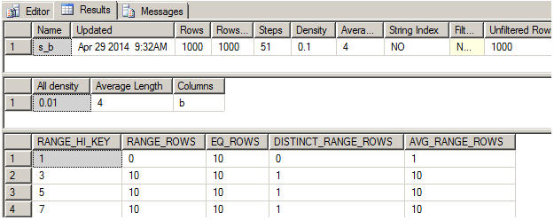
If the optimizer needs to know how the specific value, let’s say 5 in the column b, is distributed, it should look into the histogram (the last dataset in the picture), find the histogram step, which the value 5 belongs to, it would be the third one, in our case. Then look if the value 5 equals to the upper border. In our case it does – we look for 5 and RANGE_HI_KEY also equals 5. If equals, then look into the EQ_ROWS (number of rows in the step that are equal to the upper border) and determine 10 rows.
The density might be used to estimate the number of distinct values in the column b, that is useful to estimate the number of rows after a grouping operation.
There is a good description of DBCC SHOW_STATISTICS command in the documentation, with a lot of details, explanation, examples and even illustrations, so I will not delve too much into it’s usage here. If you are not familiar with it, I encourage you to visit the related link at the end of this post.
Basic statistic is a very interesting topic, there are many pitfalls and nuances. The whole book chapters or even books are dedicated exactly to that topic. It absolutely deserves it, because a lot of performance problems might be solved, if you know how to deal with statistics. But the focus of this blog post is not the statistics itself, but how it is used for the estimation, and so I’ll not make any deep dives into that topic, leaving it for the probable future posts.
The base statistics used by the optimizer to get some initial data, but what happens next – next the mathematical model is in charge.
The Model
The optimizer uses the mathematical model over the base statistics to perform an estimate. The mathematical model includes three main parts:
- Probability theory
- Assumptions
- Guesses
Let’s take a quick look at each of them using the database “opt”.
Probability theory
Assume that we have a simple query
|
1 |
select * from t1 where b = 1 |
How can the optimizer predict the number of rows returned by this query? On the first step, it uses the base statistics and table metadata. From the table metadata, it knows that table contains 1000 rows, i.e. the base cardinality is 1000 rows. The base statistics distribution histogram for the column “b” reflects the column value distribution, and the optimizer may use it to know, that there are 10 rows equal to 1.
Now, ask yourself a question – what is the probability to take a red shoe from the box with one thousand shoes of different colors, if we know that there are ten red shoes in this box? The answer is quite intuitive we should divide 10 by 1000. I.e. take all the events that may lead to the desired result (pick the red shoe – total 10), and divide them by the number of all the possible events (pick every shoe – total 1000). The number 10/1000 = 0.01 is the probability of the predicate to be true.
The predicate is defined as an expression that might be either true or false, for example, in the expression “where b=1 and c=2” – “b=1” is a predicate, “c=2” is also a predicate, and “b=1 and c=2” is a complex predicate.
The probability of the predicate to be either true or false is called a selectivity of the predicate.
We are now back from the probability theory to SQL and, using that knowledge, we may say that the selectivity of the predicate in the WHERE clause “b=1” is 0.01 percent. To get the estimated cardinality, we should multiply that selectivity by the table cardinality and we’ll get a perfect 10 rows estimate.
Now, assume that we want to know the probability of picking the red left shoe. There are two independent events: “pick the left shoe” and “pick the red shoe”. These are two independent events and the probability theory says that their complex probability should be calculated as a multiplication of the two probabilities. It seems quite intuitive, the more complex event you consider – the less is the probability. For example, one man can sneeze, and one dog can bark, very common things – but what is the probability if one man walking down the street sneezes and the dog barks exactly at the same time – quite low, however, it happens.
The logic of multiplication the probabilities was applied to the complex filtering predicates prior to SQL Server 2014 by default. The simple predicates were assumed to be independent and their selectivities were multiplied to evaluate the complex predicate selectivity, however, in real life, the data stored in the columns is not so independent. This independence assumption was relaxed in 2014 SQL Server and we will talk about it in the next posts, what is important now – we got to know, how the probability theory is applied, and even touched the next topic – assumptions.
Assumptions
Assumptions are made about the data and its distribution. We have already talked about the independence assumption for the columns. This is one of the most vulnerable assumptions and often is not true. It is so vulnerable that Microsoft even produced a trace flag 4137 to leverage this assumption, this flag forces the optimizer to use minimum selectivity instead of selectivity multiplication if multiple column predicates are involved.
Below I’ll list main assumptions with a brief description. We will not discuss them here in details, however, will definitely return to them in future posts.
- Uniformity assumption – when distribution for a column is unknown, uniformity is assumed. The uniformity assumption is used when the histogram is not available or inside of a histogram step, where the value distribution is also unknown.
- Independence assumption – columns considered to be independent, unless the correlation between them is known (e.g. multicolumn statistics is created). This is what we have talked about and in general this is a legacy assumption that was changed by default in SQL Server 2014, however, it is still used even in 2014 for some estimates.
- Inclusion assumption – when comparing a column with a constant inside histogram boundaries, it is assumed that there is always a match. The number of matched rows is assumed to be equal to a density multiplied by cardinality of a histogram step, i.e. the average frequency of a histogram step. If it is not possible to use histogram the average column density is used to calculate the average frequency.
- Containment assumption – when comparing two columns it is assumed that a column containing more distinct values contains all the distinct values from the other column. It is often used in the join estimation when combining and aligning histograms.
We will not deep dive in the assumptions here, but it is worth to say that a lot of them has changed or, to be more correct, the default assumption application has changed. We’ll leave it for the future topic.
Guesses
When there are no statistics available or it cannot be used, the optimizer has to guess. One of the most important guesses is inequality (“>” or “<“) with the unknown (local variable, for example). In this case, 30% selectivity guess is made. That means that 30% of table rows are expected to be returned from the table.
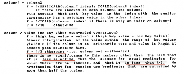
I wondered – why 30%? Not 20, not 40, but 30! And the eldest document I’ve found was the document from the 1979 from IBM – ” Access Path Selection in a Relational Database Management System “. Below you may see an explanation of 30% guess.
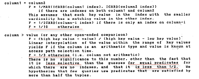
The explanation sounds a little bit naive, however, it is used up to these days.
Among the other guesses, we may name 1 row for a table variable, 1 row for a multi-statement table function (changed in SQL Server 2014), 10% compared with the unknown value, where statistics is not available and a few more.
I think now we have a background for the further talk about some estimation details.
Table of Contents
References
- Statistics
- DBCC SHOW_STATISTICS (Transact-SQL)
- Understanding SQL Server Cardinality Estimations by Charting Histogram to Actual Values
- SQL Server Statistics: Charting Volatile Data And Density Vector Values

Currently he works as a database developer lead, responsible for the development of production databases in a media research company. He is also an occasional speaker at various community events and tech conferences. His favorite topic to present is about the Query Processor and anything related to it. Dmitry is a Microsoft MVP for Data Platform since 2014.
View all posts by Dmitry Piliugin
- SQL Server 2017: Adaptive Join Internals - April 30, 2018
- SQL Server 2017: How to Get a Parallel Plan - April 28, 2018
- SQL Server 2017: Statistics to Compile a Query Plan - April 28, 2018