

In this note, I’m going to discuss one of the most useful and helpful cardinality estimator enhancements – the Ascending Key estimation.
We should start with defining the problem with the ascending keys and then move to the solution, provided by the new CE.
Ascending Key is a common data pattern and you can find it in an almost every database. These might be: identity columns, various surrogate increasing keys, date columns where some point in time is fixed (order date or sale date, for instance) or something like this – the key point is, that each new portion of such data has the values that are greater than the previous values.
As we remember, the Optimizer uses base statistics to estimate the expected number of rows returned by the query, distribution histogram helps to determine the value distribution and predict the number of rows. In various RDBMS various types of histograms might be used for that purpose, SQL Server uses a Maxdiff histogram. The histogram building algorithm builds histogram’s steps iteratively, using the sorted attribute input (the exact description of that algorithm is beyond the scope of this note, however, it is curious, and you may read the patent US 6714938 B1 – “Query planning using a maxdiff histogram” for the details, if interested). What is important that at the end of this process the histogram steps are sorted in ascending order. Now imagine, that some portion of the new data is loaded, and this portion is not big enough to exceed the automatic update statistic threshold of 20% (especially, this is the case when you have a rather big table with several millions of rows), i.e. the statistics are not updated.
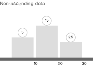
In the case of the non-ascending data, the newly added data may be more or less accurate considered by the Optimizer with the existing histogram steps, because each new row will belong to some of the histogram’s steps and there is no problem.
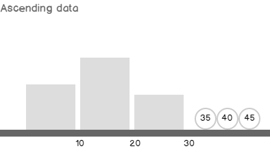
If the data has ascending nature, then it becomes a problem. The histogram steps are ascending and the maximum step reflects the maximum value before the new data was loaded. The loaded data values are all greater than the maximum old value because the data has ascending nature, so they are also greater than the maximum histogram step, and so will be beyond the histogram scope.
The way how this situation is treated in the new CE and in the old CE is a subject of this note. Now, it is time to look at the example.
We will use the AdventureWorks2012 database, but not to spoil the data with modifications, I’ll make a copy of the tables of interest and their indexes.
|
1 2 3 4 5 6 7 8 9 10 11 12 13 14 15 16 17 18 19 |
use AdventureWorks2012; ------------------------------------------------ -- Prepare Data if object_id('dbo.SalesOrderHeader') is not null drop table dbo.SalesOrderHeader; if object_id('dbo.SalesOrderDetail') is not null drop table dbo.SalesOrderDetail; select * into dbo.SalesOrderHeader from Sales.SalesOrderHeader; select * into dbo.SalesOrderDetail from Sales.SalesOrderDetail; go alter table dbo.SalesOrderHeader add constraint PK_DBO_SalesOrderHeader_SalesOrderID primary key clustered (SalesOrderID) create unique index AK_SalesOrderHeader_rowguid on dbo.SalesOrderHeader(rowguid) create unique index AK_SalesOrderHeader_SalesOrderNumber on dbo.SalesOrderHeader(SalesOrderNumber) create index IX_SalesOrderHeader_CustomerID on dbo.SalesOrderHeader(CustomerID) create index IX_SalesOrderHeader_SalesPersonID on dbo.SalesOrderHeader(SalesPersonID) alter table dbo.SalesOrderDetail add constraint PK_DBO_SalesOrderDetail_SalesOrderID_SalesOrderDetailID primary key clustered (SalesOrderID, SalesOrderDetailID); create index IX_SalesOrderDetail_ProductID on dbo.SalesOrderDetail(ProductID); create unique index AK_SalesOrderDetail_rowguid on dbo.SalesOrderDetail(rowguid); create index ix_OrderDate on dbo.SalesOrderHeader(OrderDate) -- * go |
Now, let’s make a query, that asks for some order information for the last month, together with the customer and some other details. I’ll also turn on statistics time metrics, because we will see the performance difference, even in such a small database. Pay attention, that TF 9481 is used to force the old cardinality estimation behavior.
|
1 2 3 4 5 6 7 8 9 10 11 12 13 14 15 16 17 18 19 20 21 22 23 24 25 26 27 28 29 30 |
-- Query set statistics time, xml on select soh.OrderDate, soh.TotalDue, soh.Status, OrderQty = sum(sod.OrderQty), c.AccountNumber, st.Name, so.DiscountPct from dbo.SalesOrderHeader soh join dbo.SalesOrderDetail sod on soh.SalesOrderID = sod.SalesOrderDetailID join Sales.Customer c on soh.CustomerID = c.CustomerID join Sales.SalesTerritory st on c.TerritoryID = st.TerritoryID left join Sales.SpecialOffer so on sod.SpecialOfferID = so.SpecialOfferID where soh.OrderDate > '20080701' group by soh.OrderDate, soh.TotalDue, soh.Status, c.AccountNumber, st.Name, so.DiscountPct order by soh.OrderDate option(querytraceon 9481) set statistics time, xml off go |
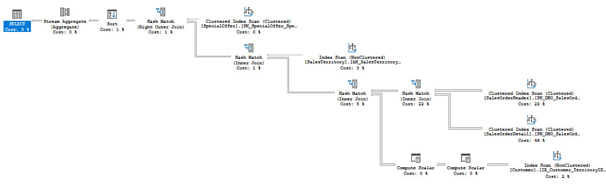
The query took 250 ms on average on my machine, and produced the following plan with Hash Joins:
Now, let’s emulate the data load, as there were some new orders for the next month saved.
|
1 2 3 4 5 6 7 8 9 10 11 12 13 14 15 16 17 18 19 20 21 22 |
-- Load Orders And Details declare @OrderCopyRelations table(SalesOrderID_old int, SalesOrderID_new int) merge dbo.SalesOrderHeader dst using ( select SalesOrderID, OrderDate = dateadd(mm,1,OrderDate), RevisionNumber, DueDate, ShipDate, Status, OnlineOrderFlag, SalesOrderNumber = SalesOrderNumber+'new', PurchaseOrderNumber, AccountNumber, CustomerID, SalesPersonID, TerritoryID, BillToAddressID, ShipToAddressID, ShipMethodID, CreditCardID, CreditCardApprovalCode, CurrencyRateID, SubTotal, TaxAmt, Freight, TotalDue, Comment, ModifiedDate from Sales.SalesOrderHeader where OrderDate > '20080701' ) src on 0=1 when not matched then insert (OrderDate, RevisionNumber, DueDate, ShipDate, Status, OnlineOrderFlag, SalesOrderNumber, PurchaseOrderNumber, AccountNumber, CustomerID, SalesPersonID, TerritoryID, BillToAddressID, ShipToAddressID, ShipMethodID, CreditCardID, CreditCardApprovalCode, CurrencyRateID, SubTotal, TaxAmt, Freight, TotalDue, Comment, ModifiedDate, rowguid) values (OrderDate, RevisionNumber, DueDate, ShipDate, Status, OnlineOrderFlag, SalesOrderNumber, PurchaseOrderNumber, AccountNumber, CustomerID, SalesPersonID, TerritoryID, BillToAddressID, ShipToAddressID, ShipMethodID, CreditCardID, CreditCardApprovalCode, CurrencyRateID, SubTotal, TaxAmt, Freight, TotalDue, Comment, ModifiedDate, newid()) output src.SalesOrderID, inserted.SalesOrderID into @OrderCopyRelations(SalesOrderID_old, SalesOrderID_new); insert dbo.SalesOrderDetail(SalesOrderID, CarrierTrackingNumber, OrderQty, ProductID, SpecialOfferID, UnitPrice, UnitPriceDiscount, LineTotal, ModifiedDate, rowguid) select ocr.SalesOrderID_new, CarrierTrackingNumber, OrderQty, ProductID, SpecialOfferID, UnitPrice, UnitPriceDiscount, LineTotal, ModifiedDate, newid() from @OrderCopyRelations ocr join Sales.SalesOrderDetail op on ocr.SalesOrderID_old = op.SalesOrderID go |
Not too much data was added: 939 rows for orders and 2130 rows for order details. That is not enough to exceed the 20% threshold for auto-update statistics.
Now, let’s repeat the previous query, and ask the orders for the last month (that would be the new added orders).
|
1 2 3 4 5 6 7 8 9 10 11 12 13 14 15 16 17 18 19 20 21 22 23 24 25 26 27 28 29 30 |
-- Old set statistics time, xml on select soh.OrderDate, soh.TotalDue, soh.Status, OrderQty = sum(sod.OrderQty), c.AccountNumber, st.Name, so.DiscountPct from dbo.SalesOrderHeader soh join dbo.SalesOrderDetail sod on soh.SalesOrderID = sod.SalesOrderDetailID join Sales.Customer c on soh.CustomerID = c.CustomerID join Sales.SalesTerritory st on c.TerritoryID = st.TerritoryID left join Sales.SpecialOffer so on sod.SpecialOfferID = so.SpecialOfferID where soh.OrderDate > '20080801' group by soh.OrderDate, soh.TotalDue, soh.Status, c.AccountNumber, st.Name, so.DiscountPct order by soh.OrderDate option(querytraceon 9481) set statistics time, xml off go |
That took 17 500 ms on average on my machine, more than 50X times slower! If you look at the plan, you’ll see that a server now using the Nested Loops Join:
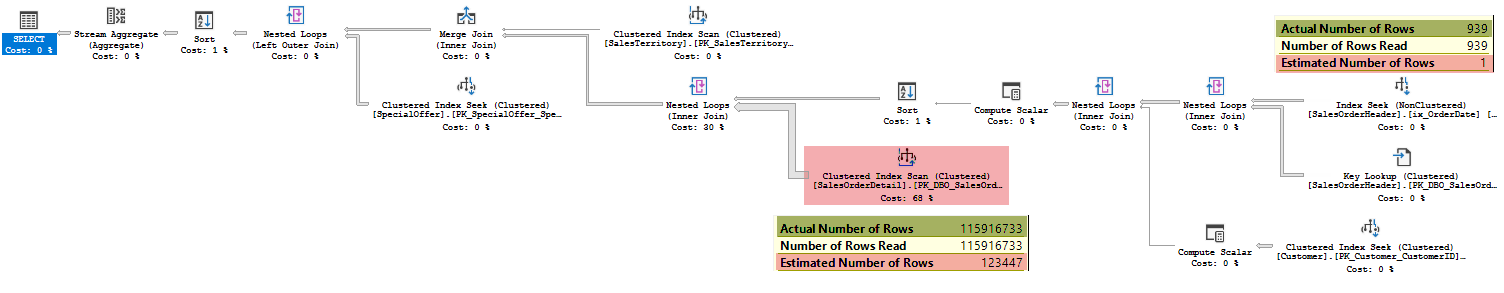
The reason for that plan shape and slow execution is the 1 row estimate, whereas 939 rows actually returned. That estimate skewed the next operator estimates. The Nested Loops Join input estimate is one row, and the optimizer decided to put the SalesOrderDetail table on the inner side of the Nested Loops – which resulted in more than 100 million of rows to be read!
CE 7.0 Solution (Pre SQL Server 2014)
To address this issue Microsoft has made two trace flags: TF 2389 and TF 2390. The first one enables statistic correction for the columns marked ascending, the second one adds other columns. More comprehensive description of those flags is provided in the post Ascending Keys and Auto Quick Corrected Statistics by Ian Jose. To see the column’s nature, you may use the undocumented TF 2388 and DBCC SHOW_STATISTICS command like this:
|
1 2 3 4 |
-- view column leading type dbcc traceon(2388) dbcc show_statistics ('dbo.SalesOrderHeader', 'ix_OrderDate') dbcc traceoff(2388) |
In this case, no surprise, the column leading type is Unknown, 3 other inserts and update statistics should be done to brand the column.

You may find a good description of this mechanism in the blog post Statistics on Ascending Columns by Fabiano Amorim. As the column branded Unknown we should use both TFs in the old CE to solve the ascending key problem.
|
1 2 3 4 5 6 7 8 9 10 11 12 13 14 15 16 17 18 19 20 21 22 23 24 25 26 27 28 29 30 |
-- Old with TFs set statistics time, xml on select soh.OrderDate, soh.TotalDue, soh.Status, OrderQty = sum(sod.OrderQty), c.AccountNumber, st.Name, so.DiscountPct from dbo.SalesOrderHeader soh join dbo.SalesOrderDetail sod on soh.SalesOrderID = sod.SalesOrderDetailID join Sales.Customer c on soh.CustomerID = c.CustomerID join Sales.SalesTerritory st on c.TerritoryID = st.TerritoryID left join Sales.SpecialOffer so on sod.SpecialOfferID = so.SpecialOfferID where soh.OrderDate > '20080801' group by soh.OrderDate, soh.TotalDue, soh.Status, c.AccountNumber, st.Name, so.DiscountPct order by soh.OrderDate option(querytraceon 9481, querytraceon 2389, querytraceon 2390) set statistics time, xml off go |
This query took the same 250 ms on average on my machine and resulted in the similar plan shape (won’t provide it here, for the space saving). Cool, isn’t it? Yes, it is, in this synthetic example.
If you are persistent enough, try to re-run the whole example from the very beginning, commenting the index ix_OrderDate creation (the one marked with the * symbol in the creation script). You will be quite surprised, that those TFs are not helpful in case of the missing index! This is a documented behavior (KB 922063):
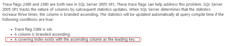
That means, that automatically created statistics (and I think in most of the real world scenarios the statistics are created automatically) won’t benefit from using these TFs.
CE 12.0 Solution (SQL Server 2014)
To address the issue of Ascending Key in SQL Server 2014 you should do… nothing! This model enhancement is turned on by default, and I think it is great! If we simply run the previous query without any TF, i.e. using the new CE, it will run like a charm. Also, no restriction of having a defined index on that column.
|
1 2 3 4 5 6 7 8 9 10 11 12 13 14 15 16 17 18 19 20 21 22 23 24 25 26 27 28 29 |
-- New set statistics time, xml on select soh.OrderDate, soh.TotalDue, soh.Status, OrderQty = sum(sod.OrderQty), c.AccountNumber, st.Name, so.DiscountPct from dbo.SalesOrderHeader soh join dbo.SalesOrderDetail sod on soh.SalesOrderID = sod.SalesOrderDetailID join Sales.Customer c on soh.CustomerID = c.CustomerID join Sales.SalesTerritory st on c.TerritoryID = st.TerritoryID left join Sales.SpecialOffer so on sod.SpecialOfferID = so.SpecialOfferID where soh.OrderDate > '20080801' group by soh.OrderDate, soh.TotalDue, soh.Status, c.AccountNumber, st.Name, so.DiscountPct order by soh.OrderDate set statistics time, xml off go |
The plan would be the following (adjusted a little bit to fit the page):
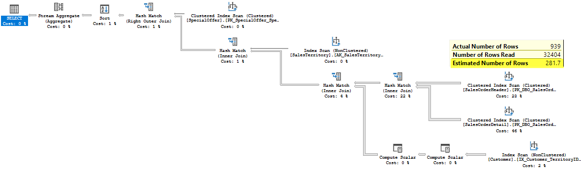
You may see that the estimated number of rows is not 1 row any more. It is 281.7 rows. That estimate leads to an appropriate plan with Hash Joins, that we saw earlier. If you wonder how this estimation was made – the answer is that in CE 2014 the “out-of-boundaries” values are modeled to belong an average histogram step (trivial histogram step with a uniform data distribution) in case of equality – it is well described in Joe Sack blog post mentioned above. In case of inequality the 30% guess, over the added rows is made (common 30% guess was discussed earlier).
|
1 |
select rowmodctr*0.3 from sys.sysindexes i where i.name = 'PK_DBO_SalesOrderHeader_SalesOrderID' |
The result is 939*0.3 = 281.7 rows. Of course a server uses another, per-column counters, but in this case it doesn’t matter. What is matter that this really cool feature is present in the new CE 2014!
Another interesting thing to note is some internals. If you run the query with the TF 2363 (and the TF 3604 of course) to view diagnostic output, you’ll see that the specific calculator CSelCalcAscendingKeyFilter is used.
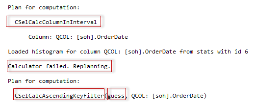
According to this output, at first the regular calculator for an inequality (or equality with non-unique column) was used. When it estimated zero selectivity, the estimation process realized that some extra steps should be done and re-planed the calculation. I think this is a result of separating the two processes, the planning for computation and the actual computation, however, I’m not sure and need some information from the inside about that architecture enhancement. The re-planed calculator is CSelCalcAscendingKeyFilter calculator that models “out-of-histogram-boundaries” distribution. You may also notice the guess argument, that stands for the 30% guess.
The Model Variation
The model variation in that case would be to turn off the ascending key logic. Besides, this is completely undocumented and should not be used in production, I strongly don’t recommend to turn off this splendid mechanism, it’s like buying a ticket and staying at home.
However, maybe this opportunity will be helpful for some geeky people (like me=)) in their optimizer experiments. To enable the model variation and turn off the ascending key logic you should run the query together with TF 9489.
|
1 2 3 4 5 6 7 8 9 10 11 12 13 14 15 16 17 18 19 20 21 22 23 24 25 26 27 28 29 |
set statistics time, xml on select soh.OrderDate, soh.TotalDue, soh.Status, OrderQty = sum(sod.OrderQty), c.AccountNumber, st.Name, so.DiscountPct from dbo.SalesOrderHeader soh join dbo.SalesOrderDetail sod on soh.SalesOrderID = sod.SalesOrderDetailID join Sales.Customer c on soh.CustomerID = c.CustomerID join Sales.SalesTerritory st on c.TerritoryID = st.TerritoryID left join Sales.SpecialOffer so on sod.SpecialOfferID = so.SpecialOfferID where soh.OrderDate > '20080801' group by soh.OrderDate, soh.TotalDue, soh.Status, c.AccountNumber, st.Name, so.DiscountPct order by soh.OrderDate option(querytraceon 9489) set statistics time, xml off go |
And with TF 9489 we are now back to the nasty Nested Loops plan. I’m sure, due to the statistical nature of the estimation algorithms you may invent the case where this TF will be helpful, but in the real world, please, don’t use it, of course, unless you are guided by Microsoft support!
That’s all for that post! Next time we will talk about multi-statement table valued functions.
Table of contents
References
- Optimizing Your Query Plans with the SQL Server 2014 Cardinality Estimator
- Ascending Keys and Auto Quick Corrected Statistics
- Optimizing Your Query Plans with the SQL Server 2014 Cardinality Estimator
- Regularly Update Statistics for Ascending Keys

Currently he works as a database developer lead, responsible for the development of production databases in a media research company. He is also an occasional speaker at various community events and tech conferences. His favorite topic to present is about the Query Processor and anything related to it. Dmitry is a Microsoft MVP for Data Platform since 2014.
View all posts by Dmitry Piliugin
- SQL Server 2017: Adaptive Join Internals - April 30, 2018
- SQL Server 2017: How to Get a Parallel Plan - April 28, 2018
- SQL Server 2017: Statistics to Compile a Query Plan - April 28, 2018