Data boundaries: Finding gaps, islands, and more

One of the more difficult challenges we face when analyzing data is to effectively identify and report on boundaries. Data sets can contain any number of significant starting and stopping points that may indicate significant events, such as missing data, important business events, or actionable changes in usage. Regardless of the use case, knowing how to quickly locate and manage data boundaries is extremely useful. Knowing how to design solutions that can effectively avoid these scenarios can also be helpful in the long run.

Sales Performance

There are many applications in which we want to return summary data that indicates the overall continuity of the data within a table. Whether interested in the exceptions where rows are missing, or the size and shape of data groups, the solutions to this problem can a challenge without a framework to divide these problems into smaller, simpler solutions. In addition, many demos of these problems offer very simplistic or trivial use cases. Our goal here is to recreate a few realistic scenarios in which determining specific boundary data for a result set can be a worthwhile task.

Let’s create an example using data from AdventureWorks using their sales data. Let’s say we were in charge of looking at sales trends over time and determined that any day where we sell less than $10,000 is significant and should be investigated further. If our company were performing optimally, there would never be a date for which our sales are below this amount. Running this query would return a row per day, including sales totals for the period of time tracked in these tables:

SELECT

OrderDate,

SUM(SubTotal) AS Daily_Order_Total

FROM Sales.SalesOrderHeader

WHERE OrderDate BETWEEN '2005-07-01' AND '2008-07-31'

GROUP BY OrderDate

ORDER BY OrderDate ASC;

Any real data set has variations in it, and here we will find days where we sell ten times the limit defined above, and others where we cannot make even half of it. We can chart this data to show the ups and downs, but there use in understanding how sales group together. With that data, we can answer questions such as, “How many days in a row, on average, do we exceed our goal?” “When we fall below the goal, how many days do we do so for?” and “What is the average time that passes from one sales failure to the next?”

To construct a solution that could answer these and many other questions, we must build a summary data set based on the parameters we defined above. One way to parse this data would be to create a list of all days in which sales did not reach the goal:

WITH CTE_SALES AS (

SELECT

OrderDate,

SUM(SubTotal) AS Daily_Order_Total

FROM Sales.SalesOrderHeader

WHERE OrderDate BETWEEN '2005-07-01' AND '2008-07-31'

GROUP BY OrderDate)

SELECT

OrderDate

FROM CTE_SALES

WHERE Daily_Order_Total < 10000

ORDER BY OrderDate ASC;

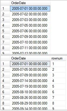
This returns a list of dates, in order, for which daily sales were under $10k:

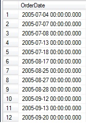
$C:\Users\epollack\Dropbox\SQL\Articles\Gaps, Islands, and Other Challenges\1_Sales_Under_Limit_List.jpg$

A total of 137 rows were returned, and while this is useful data, it doesn’t answer very many questions without further analysis. From this point, we can put that data into a temporary table and analyze further, or we can find a set-based solution that provides what we want in a single step. For this problem, we will do both!

Let’s say that we placed the above results into a temporary table called #order_dates and to start, we want to summarize the data into a set of dates indicating any periods of time in which the sales goal was not met. In order to do this effectively, we need to be able to order these dates and determine how far from the starting date each one is. By collecting this data, we can determine which dates are adjacent and comprise a period of poor sales, which dates stand alone, and which periods have no corresponding rows. To allow for cleaner TSQL, we’ll put the start and end dates for our data set into scalar variables, which could later be parameterized to ensure good performance:

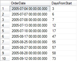
DECLARE @start_date DATE = '2005-07-01';

DECLARE @end_date DATE = '2008-07-31';

SELECT

OrderDate,

DATEDIFF(DAY, @start_date, OrderDate) AS DaysFromStart

FROM #order_dates

ORDER BY OrderDate

The result set provides a relationship between the start date for our data and any given row:

$C:\Users\epollack\Dropbox\SQL\Articles\Gaps, Islands, and Other Challenges\2_Sales_Demo_Days_From_Start.jpg$

Using this information, we can compare this measurement of days from the start of our data with its relative position within the set. The result will be a numeric identifier that is identical for any adjacent rows that occur for consecutive days:

WITH CTE_DAYSFROMSTART AS (

SELECT

OrderDate,

DATEDIFF(DAY, @start_date, OrderDate) AS DaysFromStart

FROM #order_dates)

SELECT

OrderDate,

DaysFromStart,

ROW_NUMBER() OVER (ORDER BY DaysFromStart) AS rownum,

DaysFromStart - ROW_NUMBER() OVER (ORDER BY DaysFromStart) AS OffsetDays

FROM CTE_DAYSFROMSTART

The results show the DaysFromStart value that we created earlier, as well as a row number, and the difference between these values:

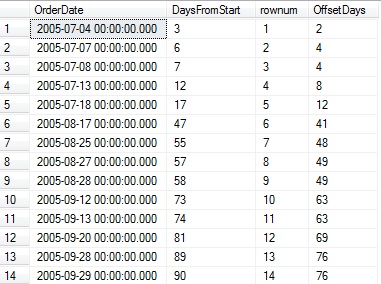
$C:\Users\epollack\Dropbox\SQL\Articles\Gaps, Islands, and Other Challenges\3_Sales_Demo_OffsetDays.jpg$

Note that whenever there are two consecutive days in the list, OffSetDays is equal for those rows. This is the basis for tying together these queries into a set of common table expressions that can solve our original question:

WITH CTE_DAYSFROMSTART AS (

SELECT

OrderDate,

DATEDIFF(DAY, @start_date, OrderDate) AS DaysFromStart

FROM #order_dates),

CTE_DATEDIFF AS (

SELECT

OrderDate,

DaysFromStart,

DaysFromStart - ROW_NUMBER() OVER (ORDER BY DaysFromStart) AS OffsetDays

FROM CTE_DAYSFROMSTART)

SELECT

DATEADD(DAY, MIN(DaysFromStart), @start_date) AS StartDate,

DATEADD(DAY, MAX(DaysFromStart), @start_date) AS EndDate

FROM CTE_DATEDIFF

GROUP BY OffsetDays;

Since OffsetDays is in chronological order, grouping by it allows us to analyze each individual set of rows that share a value. For each subset, the minimum and maximum values will provide a start and end date for each block of dates:

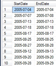
$C:\Users\epollack\Dropbox\SQL\Articles\Gaps, Islands, and Other Challenges\4_Sales_Demo_Results.jpg$

The end result is a set of date ranges, each of which identify a day or days in which sales were below our threshold of $10k for any particular day. If we’d like to remove a CTE and shorten the above TSQL a bit, we can roll the definition of DaysFromStart into the remainder of the query:

WITH CTE_DATEDIFF AS (

SELECT

OrderDate,

DATEDIFF(DAY, @start_date, OrderDate) AS DaysFromStart,

DATEDIFF(DAY, @start_date, OrderDate) - ROW_NUMBER() OVER (ORDER BY DATEDIFF(DAY, @start_date, OrderDate)) AS OffsetDays

FROM #order_dates)

SELECT

DATEADD(DAY, MIN(DaysFromStart), @start_date) AS StartDate,

DATEADD(DAY, MAX(DaysFromStart), @start_date) AS EndDate

FROM CTE_DATEDIFF

GROUP BY OffsetDays;

This query is logically equivalent to the previous one, and also performs similarly. It is also possible to solve this problem using the original data, without storing the results in a temporary table:

WITH CTE_SALES AS (

SELECT

OrderDate,

SUM(SubTotal) AS Daily_Order_Total

FROM Sales.SalesOrderHeader

WHERE OrderDate BETWEEN @start_date AND @end_date

GROUP BY OrderDate),

CTE_DATEDIFF AS (

SELECT

OrderDate,

DATEDIFF(DAY, @start_date, OrderDate) AS DaysFromStart,

DATEDIFF(DAY, @start_date, OrderDate) - ROW_NUMBER() OVER (ORDER BY DATEDIFF(DAY, @start_date, OrderDate)) AS OffsetDays

FROM CTE_SALES

WHERE Daily_Order_Total < 10000)

SELECT

DATEADD(DAY, MIN(DaysFromStart), @start_date) AS StartDate,

DATEADD(DAY, MAX(DaysFromStart), @start_date) AS EndDate

FROM CTE_DATEDIFF

GROUP BY OffsetDays;

As before, the results are equivalent, and performance of each of these options is also similar. Which one to use would depend on readability, as well as if we’d like to reuse the temp table for any other operations.

There are other ways to solve this problem. For example, if we wanted to get a list of all date ranges in which we did meet our sales goal, we could create start points and end points as we did above, but in separate steps:

DECLARE @start_date DATE = '2005-07-01';

DECLARE @end_date DATE = '2008-07-31';

SELECT

OrderDate

FROM Sales.SalesOrderHeader

WHERE OrderDate BETWEEN @start_date AND @end_date

GROUP BY OrderDate

HAVING SUM(SubTotal) >= 10000

order by OrderDate;

WITH CTE_SALES AS (

SELECT

OrderDate

FROM Sales.SalesOrderHeader

WHERE OrderDate BETWEEN @start_date AND @end_date

GROUP BY OrderDate

HAVING SUM(SubTotal) >= 10000),

CTE_StartDates AS (

SELECT

OrderDate,

ROW_NUMBER() OVER (ORDER BY OrderDate) AS rownum

FROM CTE_SALES AS SalesBaseDay

WHERE NOT EXISTS (

SELECT

FROM CTE_SALES AS SalesAdjacentDay

WHERE DATEDIFF(DAY, SalesAdjacentDay.OrderDate, SalesBaseDay.OrderDate) = 1))

SELECT

FROM CTE_StartDates

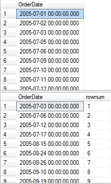
CTE_StartDates selects from the same base data set that we worked with earlier, but performs an existence check to determine if an adjacent row exists after the current row. The original data is selected above this to serve as a reference:

$C:\Users\epollack\Dropbox\SQL\Articles\Gaps, Islands, and Other Challenges\5_Sales_Demo_StartDates.jpg$

Note the breaks in the OrderDate list that signify days in which the sales goal was not met and the corresponding rows below that indicate the start of each continuous set of days in which the goal was met. We can perform an almost identical task in order to retrieve the end dates for each group of days by changing the DATEDIFF to check for -1 rather than 1:

WHERE DATEDIFF(DAY, SalesAdjacentDay.OrderDate, SalesBaseDay.OrderDate) = -1))

The results are as follows:

$C:\Users\epollack\Dropbox\SQL\Articles\Gaps, Islands, and Other Challenges\6_Sales_Demo_EndDates.jpg$

Note that each row in the second result set corresponds to the end of a set of good sales days in the first result set. With starting and ending points defined, the task of combining them is the same as it was in the previous analysis:

DECLARE @start_date DATE = '2005-07-01';

DECLARE @end_date DATE = '2008-07-31';

WITH CTE_SALES AS (

SELECT

OrderDate

FROM Sales.SalesOrderHeader

WHERE OrderDate BETWEEN @start_date AND @end_date

GROUP BY OrderDate

HAVING SUM(SubTotal) >= 10000),

CTE_StartDates AS (

SELECT

OrderDate,

ROW_NUMBER() OVER (ORDER BY OrderDate) AS rownum

FROM CTE_SALES AS SalesBaseDay

WHERE NOT EXISTS (

SELECT

FROM CTE_SALES AS SalesAdjacentDay

WHERE DATEDIFF(DAY, SalesAdjacentDay.OrderDate, SalesBaseDay.OrderDate) = 1)),

CTE_EndDates AS (

SELECT

OrderDate,

ROW_NUMBER() OVER (ORDER BY OrderDate) AS rownum

FROM CTE_SALES AS SalesBaseDay

WHERE NOT EXISTS (

SELECT

FROM CTE_SALES AS SalesAdjacentDay

WHERE DATEDIFF(DAY, SalesAdjacentDay.OrderDate, SalesBaseDay.OrderDate) = -1))

SELECT

CTE_StartDates.OrderDate AS StartDate,

CTE_EndDates.OrderDate AS EndDate

FROM CTE_StartDates

INNER JOIN CTE_EndDates

ON CTE_StartDates.rownum = CTE_EndDates.rownum

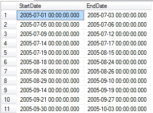
By joining each set of dates based on the row number, we end up with the inverse of the StartDate/EndDate list from earlier. This time we report on the dates in which sales met the goal, rather than those dates where it wasn’t achieved:

$C:\Users\epollack\Dropbox\SQL\Articles\Gaps, Islands, and Other Challenges\7_Sales_Demo_Results2.jpg$

Given this data, we can determine a huge variety of metrics that could be useful for further analysis. Each of these metrics can be used in place of the final SELECT statement above:

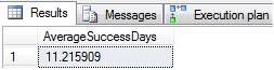
Average length in days in a successful sales streak:

SELECT

AVG(CAST(DATEDIFF(DAY, CTE_StartDates.OrderDate, CTE_EndDates.OrderDate) + 1 AS DECIMAL)) AS AverageSuccessDays

FROM CTE_StartDates

INNER JOIN CTE_EndDates

ON CTE_StartDates.rownum = CTE_EndDates.rownum

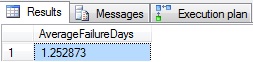
$C:\Users\epollack\Dropbox\SQL\Articles\Gaps, Islands, and Other Challenges\8_Sales_Demo_Avg_Success_Days.jpg$

Average length in days of unsuccessful sales streaks:

CTE_ISLANDS AS (

SELECT

CTE_StartDates.OrderDate AS StartDate,

CTE_EndDates.OrderDate AS EndDate,

ROW_NUMBER() OVER (ORDER BY CTE_StartDates.OrderDate ASC) AS rownum

FROM CTE_StartDates

INNER JOIN CTE_EndDates

ON CTE_StartDates.rownum = CTE_EndDates.rownum)

SELECT

AVG(CAST(DATEDIFF(DAY, LeadingRow.EndDate, LaggingRow.StartDate) - 1 AS DECIMAL)) AS AverageFailureDays

FROM CTE_ISLANDS LeadingRow

INNER JOIN CTE_ISLANDS LaggingRow

ON LaggingRow.rownum = LeadingRow.rownum + 1

$C:\Users\epollack\Dropbox\SQL\Articles\Gaps, Islands, and Other Challenges\9_Sales_Demo_Avg_Failure_Days.jpg$

Number of successful sales streaks started in each month for all data:

SELECT

DATEPART(MONTH, CTE_StartDates.OrderDate) AS StartMonth,

COUNT(DATEPART(MONTH, CTE_StartDates.OrderDate)) AS NumberOfWinningStreaksStarted

FROM CTE_StartDates

INNER JOIN CTE_EndDates

ON CTE_StartDates.rownum = CTE_EndDates.rownum

GROUP BY DATEPART(MONTH, CTE_StartDates.OrderDate)

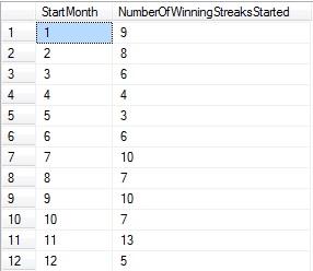
$C:\Users\epollack\Dropbox\SQL\Articles\Gaps, Islands, and Other Challenges\10_Sales_Demo_Successful_Days_By_Month.jpg$

Note that the number of winning streaks started per month is also indicative of the number of poor sales days per month. As a result, a metrics such as this may provide multiple roads for analysis.

Any of these metrics (and others) could be calculated by inserting the initial results into a temp table, in order to remove potential performance problems when nesting so many CTEs together.

Transaction History

Another scenario in which boundaries may be useful to analyze is when looking at order history for a specific product. When are the largest gaps in sales, and what events lead up to them? How do we translate specific data requests into a query for which we can analyze it as we did previously?

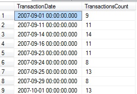
Let’s consider the situation where we are interested in mountain tire sales. Specifically, we want to understand the quantity sold per day and understand those periods in which we sell the least per day. To do this, we will create a TSQL query that filters the transaction history data specifically for mountain tires where the transaction type is a Sale, and where the number of distinct transactions is less than 15:

SELECT

TransactionHistory.TransactionDate,

COUNT(*) AS TransactionsCount

FROM Production.TransactionHistory

INNER JOIN Production.Product

ON TransactionHistory.ProductID = Product.ProductID

WHERE Product.Name LIKE '%Mountain Tire%'

AND TransactionHistory.TransactionType = 'S'

GROUP BY TransactionHistory.TransactionDate

HAVING COUNT(TransactionID) < 15

ORDER BY TransactionHistory.TransactionDate;

This returns a row with a date and the number of transactions for that particular day:

$C:\Users\epollack\Dropbox\SQL\Articles\Gaps, Islands, and Other Challenges\11_Transaction_History_Demo_Core_Data.jpg$

With this data set defined, we can turn this data into date ranges in which we provide some aggregate transaction details:

DECLARE @start_date DATE = '2007-09-01';

DECLARE @end_date DATE = '2008-07-31';

WITH CTE_TRANSACTIONS AS (

SELECT

TransactionHistory.TransactionDate,

COUNT(*) AS TransactionsCount

FROM Production.TransactionHistory

INNER JOIN Production.Product

ON TransactionHistory.ProductID = Product.ProductID

WHERE Product.Name LIKE '%Mountain Tire%'

AND TransactionHistory.TransactionType = 'S'

GROUP BY TransactionHistory.TransactionDate

HAVING COUNT(TransactionID) < 15),

CTE_DATEDIFF AS (

SELECT

TransactionDate,

DATEDIFF(DAY, @start_date, TransactionDate) AS DaysFromStart,

DATEDIFF(DAY, @start_date, TransactionDate) - ROW_NUMBER() OVER (ORDER BY DATEDIFF(DAY, @start_date, TransactionDate)) AS OffsetDays,

TransactionsCount

FROM CTE_TRANSACTIONS)

SELECT

DATEADD(DAY, MIN(DaysFromStart), @start_date) AS StartDate,

DATEADD(DAY, MAX(DaysFromStart), @start_date) AS EndDate,

SUM(TransactionsCount) AS TransactionsCount

FROM CTE_DATEDIFF

GROUP BY OffsetDays;

This query returns the groups of days in which the transaction count was under 15, as well as the number of transactions for that given period:

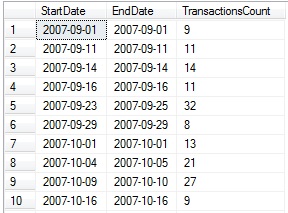
$C:\Users\epollack\Dropbox\SQL\Articles\Gaps, Islands, and Other Challenges\12_Transaction_History_Demo_Grouped_Data.jpg$

The ability to carry aggregate metrics such as count, sum, min, or max through these data transformations can be a time and resource saver later on, in the event that we need transaction counts, revenue, or other data, in addition to dates. Since Production.TransactionHistory is a large table, I will place the above results in a temporary table, #Transaction_Data, and calculate our last few metrics using this small data set instead:

Top losing streaks by fewest transactions per day:

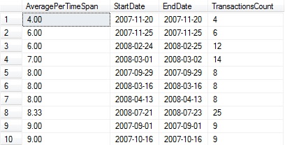
WITH CTE_AVERAGES AS (

SELECT

StartDate,

EndDate,

DATEDIFF(DAY, StartDate, EndDate) + 1 AS TimeSpan,

TransactionsCount

FROM #Transaction_Data)

SELECT TOP 10

CAST(CAST(TransactionsCount AS DECIMAL) / CAST(TimeSpan AS DECIMAL) AS DECIMAL(10,2)) AS AveragePerTimeSpan,

StartDate,

EndDate,

TransactionsCount

FROM CTE_AVERAGES

ORDER BY CAST(TransactionsCount AS DECIMAL) / CAST(TimeSpan AS DECIMAL) ASC

This returns an ordered list of the time spans with the fewest transactions:

$C:\Users\epollack\Dropbox\SQL\Articles\Gaps, Islands, and Other Challenges\13_Transaction_History_Demo_Fewest_Transactions.jpg$

Months with the most transactions accounted for via low activity periods that started in that month:

WITH CTE_MONTH_DATA AS (

SELECT

DATEPART(MONTH, StartDate) AS TransactionMonth,

TransactionsCount,

DATEDIFF(DAY, StartDate, EndDate) + 1 AS DaysIncluded

FROM #Transaction_Data

)

SELECT

TransactionMonth,

SUM(TransactionsCount) AS AggregateTransactionCount,

COUNT(*) AS NumberOfDateRanges,

SUM(DaysIncluded) AS DaysIncludedInAggregate

FROM CTE_MONTH_DATA

GROUP BY TransactionMonth

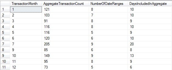
$C:\Users\epollack\Dropbox\SQL\Articles\Gaps, Islands, and Other Challenges\14_Transaction_History_Demo_Monthly_Transaction_Count_Aggregation.jpg$

Looking at this data, it would appear that the most volatile month with the largest percentage of the data appearing in low-activity periods is July, whereas December has the fewest periods of low activity. Note that August is excluded in this data as the underlying results include no entries from that month.

Baseball Statistics

There are few areas more suitable for statistical analysis than in sports, and of the many sports played around the world, few rival baseball for the volume, accuracy, and complexity of available data. Before diving into a few additional examples, let’s summarize a basic method for effectively analyzing data in order to work with data boundaries:

Determine the criteria needed to enumerate a desired boundary.
Use that criteria to order the data based on whatever dates, times, or sequences are to be analyzed.
If necessary, convert that order into an integer sequence, which will allow for much easier analysis.
Calculate start and end points for gaps or islands formed by those boundaries.
Use the resulting data ranges to calculate whatever metrics you are looking for.

Using data from Retrosheet.org, a non-profit organization that collects and makes publically available baseball statistics, I’ve created a new database called BaseballStats and loaded game log data into a new table called dbo.GameLog. This table contains a row per game played, and includes data on each team, who played, and a plethora of statistics about how the game was played. This includes everything from the name of the third base umpire to how many triples were scored by each team. The data used here covers all games played from 1871 through 2015: 212,435 games in total.

A sample of data from this table looks like this:

While this table contains 163 columns, we’ll only focus on a small subset of them, in an effort to keep this simple.

Some of the most commonly requested statistics in sports involves winning streaks. Not only are we interested in knowing how many games a team currently has won in a row, but we may also have more involved questions, such as:

What is the longest winning stream a team has had in the past 5 years?
What is the longest losing streak a team has had versus a specific other team?
How many games has a specific pitcher won in a row?
How much longer are losing streaks by a team when at least one error was made?
What is the longest winning streak by a team, at home, on Sundays, at night?

While the last one is a bit of a joke, statistical analysis of sports can get this in-depth. There are players that legitimately pitch better at night, hit more home runs after a day of rest, or hit significantly worse against lefties. Managers that are looking for an edge in a close matchup are more than happy to make minor changes for small gains overall.

For our first metric, let’s determine when the longest regular season winning streak in the history of the Yankees was, and how many games they won before their streak came to an end. In order to do this, we need to create an ordered list of games in which they played:

SELECT

CASE WHEN HomeScore > VisitingScore AND HomeTeamName = 'NYA' THEN 'W'

WHEN HomeScore > VisitingScore AND VisitingTeamName = 'NYA' THEN 'L'

WHEN VisitingScore > HomeScore AND VisitingTeamName = 'NYA' THEN 'W'

WHEN VisitingScore > HomeScore AND HomeTeamName = 'NYA' THEN 'L'

END AS Result

FROM dbo.GameLog

WHERE (HomeTeamName = 'NYA' OR VisitingTeamName = 'NYA')

AND GameType = 'REG'

ORDER BY GameDate ASC, GameNumber ASC;

This returns all 17658 games they have played in since 1903:

The Result column we create will be greatly simplify calculations later on as we’ll have an easy way to identify winning vs. losing games. With this information, we’ll build a sequence where wins signify a bounded set of interest, and losses are gaps in that data:

WITH CTE_BASEBALL_GAMES AS (

SELECT

CASE WHEN HomeScore > VisitingScore AND HomeTeamName = 'NYA' THEN 'W'

WHEN HomeScore > VisitingScore AND VisitingTeamName = 'NYA' THEN 'L'

WHEN VisitingScore > HomeScore AND VisitingTeamName = 'NYA' THEN 'W'

WHEN VisitingScore > HomeScore AND HomeTeamName = 'NYA' THEN 'L'

END AS Result,

ROW_NUMBER() OVER (ORDER BY GameDate ASC, GameNumber ASC) AS rownum

FROM dbo.GameLog

WHERE (HomeTeamName = 'NYA' OR VisitingTeamName = 'NYA')

AND GameType = 'REG'

AND (HomeScore > VisitingScore OR VisitingScore > HomeScore)),

CTE_StartofWinningStreak AS (

SELECT

ROW_NUMBER() OVER (ORDER BY GameDate ASC, GameNumber ASC) AS StartNum

FROM CTE_BASEBALL_GAMES AS GameDay

WHERE Result = 'W'

AND EXISTS (

SELECT

FROM CTE_BASEBALL_GAMES AS PreviousGame

WHERE GameDay.rownum = PreviousGame.rownum + 1

AND PreviousGame.Result = 'L')),

CTE_EndofWinningStreak AS (

SELECT

ROW_NUMBER() OVER (ORDER BY GameDate ASC, GameNumber ASC) AS EndNum

FROM CTE_BASEBALL_GAMES AS GameDay

WHERE Result = 'W'

AND EXISTS (

SELECT

FROM CTE_BASEBALL_GAMES AS NextGame

WHERE GameDay.rownum = NextGame.rownum - 1

AND NextGame.Result = 'L'))

SELECT

CTE_StartofWinningStreak.GameDate AS StartDate,

CTE_EndofWinningStreak.GameDate AS EndDate,

FROM CTE_StartofWinningStreak

INNER JOIN CTE_EndofWinningStreak

ON CTE_StartofWinningStreak.StartNum = CTE_EndofWinningStreak.EndNum

ORDER BY CTE_StartofWinningStreak.GameDate, CTE_StartofWinningStreak.GameNumber;

Our base data set (CTE_BASEBALL_GAMES) checks for only regular season games, only those where the result was a win or loss—ties are excluded. The second and third CTEs each determine a start and end boundary for each winning streak. Since multiple games can be played in a single day, we consistently order data by GameDate and GameNumber. The results of this query are the start and end dates of each winning streak, as well as all of the data associated with the starting game in the streak:

From this data set, we can calculate the length of their longest winning streak as follows:

WITH CTE_BASEBALL_GAMES AS (

SELECT

CASE WHEN HomeScore > VisitingScore AND HomeTeamName = 'NYA' THEN 'W'

WHEN HomeScore > VisitingScore AND VisitingTeamName = 'NYA' THEN 'L'

WHEN VisitingScore > HomeScore AND VisitingTeamName = 'NYA' THEN 'W'

WHEN VisitingScore > HomeScore AND HomeTeamName = 'NYA' THEN 'L'

END AS Result,

ROW_NUMBER() OVER (ORDER BY GameDate ASC, GameNumber ASC) AS rownum

FROM dbo.GameLog

WHERE (HomeTeamName = 'NYA' OR VisitingTeamName = 'NYA')

AND GameType = 'REG'

AND (HomeScore > VisitingScore OR VisitingScore > HomeScore)),

CTE_StartofWinningStreak AS (

SELECT

ROW_NUMBER() OVER (ORDER BY GameDate ASC, GameNumber ASC) AS StartNum

FROM CTE_BASEBALL_GAMES AS GameDay

WHERE Result = 'W'

AND EXISTS (

SELECT

FROM CTE_BASEBALL_GAMES AS PreviousGame

WHERE GameDay.rownum = PreviousGame.rownum + 1

AND PreviousGame.Result = 'L')),

CTE_EndofWinningStreak AS (

SELECT

ROW_NUMBER() OVER (ORDER BY GameDate ASC, GameNumber ASC) AS EndNum

FROM CTE_BASEBALL_GAMES AS GameDay

WHERE Result = 'W'

AND EXISTS (

SELECT

FROM CTE_BASEBALL_GAMES AS NextGame

WHERE GameDay.rownum = NextGame.rownum - 1

AND NextGame.Result = 'L'))

SELECT

CTE_EndofWinningStreak.rownum - CTE_StartofWinningStreak.rownum + 1 AS WinningStreak,

CTE_StartofWinningStreak.GameDate AS StartGameDate, CTE_StartofWinningStreak.GameNumber AS StartGameNumber,

CTE_EndofWinningStreak.GameDate AS EndGameDate, CTE_EndofWinningStreak.GameNumber AS EndGameNumber,

FROM CTE_StartofWinningStreak

INNER JOIN CTE_EndofWinningStreak

ON CTE_StartofWinningStreak.StartNum = CTE_EndofWinningStreak.EndNum

ORDER BY CTE_EndofWinningStreak.rownum - CTE_StartofWinningStreak.rownum DESC;

This returns all winning streaks sorted by their length, with the top winning streak appearing first in the list:

From this data, we can conclude that the longest winning streak in the history of the New York Yankees was 19 games, starting in the second game of a double header on 6/29/1947 versus the Washington Senators and ending after a double header on 7/17/1947.

Using this method, we could calculate winning streaks under any conditions by modifying the initial SELECT statement in CTE_BASEBALL_STATS, allowing us to customize the date span, filter on the presence of specific players, teams, or anything else we can dream up.

For one final example, let’s analyze pitching performance and determine the distribution of winning streaks by legend Nolan Ryan. In order to do this, we’ll need to start with a data set of all games he has pitched, flagged with whether he won or lost. The data from Retrosheet includes the names of all players on each team, as well as the winning pitcher’s name, as well as losing pitcher’s name. Using this, we can flag each game he pitched as a Win (W), Loss (L), or No decision (N). Winning streaks will only be counted if all games were won, and if Nolan Ryan started the game (games where he was brought in as a reliever won’t be included):

DECLARE @PitcherName VARCHAR(100) = 'Nolan Ryan';

SELECT

CASE WHEN WinningPitcherName = @PitcherName THEN 'W'

WHEN LosingPitcherName = @PitcherName THEN 'L'

ELSE 'N'

END AS Result,

ROW_NUMBER() OVER (ORDER BY GameDate ASC, GameNumber ASC) AS rownum,

FROM dbo.GameLog

WHERE (VisitingStartingPitcherName = @PitcherName OR HomeStartingPitcherName = @PitcherName)

ORDER BY GameDate ASC, GameNumber ASC;

The results are similar to earlier and provide win/loss details for every game that he started:

We can take this query and determine winning and losing streaks almost identically to our previous calculations for the Yankees:

DECLARE @PitcherName VARCHAR(100) = 'Nolan Ryan';

WITH CTE_PITCHING AS (

SELECT

CASE WHEN WinningPitcherName = @PitcherName THEN 'W'

WHEN LosingPitcherName = @PitcherName THEN 'L'

ELSE 'N'

END AS Result,

ROW_NUMBER() OVER (ORDER BY GameDate ASC, GameNumber ASC) AS rownum,

FROM dbo.GameLog

WHERE (VisitingStartingPitcherName = @PitcherName OR HomeStartingPitcherName = @PitcherName)),

CTE_StartofWinningStreak AS (

SELECT

ROW_NUMBER() OVER (ORDER BY GameDate ASC, GameNumber ASC) AS StartNum

FROM CTE_PITCHING AS GameDay

WHERE Result = 'W'

AND EXISTS (

SELECT

FROM CTE_PITCHING AS PreviousGame

WHERE GameDay.rownum = PreviousGame.rownum + 1

AND PreviousGame.Result <> 'W')),

CTE_EndofWinningStreak AS (

SELECT

ROW_NUMBER() OVER (ORDER BY GameDate ASC, GameNumber ASC) AS EndNum

FROM CTE_PITCHING AS GameDay

WHERE Result = 'W'

AND EXISTS (

SELECT

FROM CTE_PITCHING AS NextGame

WHERE GameDay.rownum = NextGame.rownum - 1

AND NextGame.Result <> 'W'))

SELECT

CTE_EndofWinningStreak.rownum - CTE_StartofWinningStreak.rownum + 1 AS WinningStreak,

CTE_StartofWinningStreak.GameDate AS StartGameDate, CTE_StartofWinningStreak.GameNumber AS StartGameNumber,

CTE_EndofWinningStreak.GameDate AS EndGameDate, CTE_EndofWinningStreak.GameNumber AS EndGameNumber,

FROM CTE_StartofWinningStreak

INNER JOIN CTE_EndofWinningStreak

ON CTE_StartofWinningStreak.StartNum = CTE_EndofWinningStreak.EndNum

ORDER BY CTE_EndofWinningStreak.rownum - CTE_StartofWinningStreak.rownum DESC;

The strategy is the same: Start with the core data we wish to analyze, determine the start and end points of each winning streak, then join them together to find the number of games in each streak. Once we have that data calculated, grouping it in order to get the distribution of winning streaks is a piece of cake:

DECLARE @PitcherName VARCHAR(100) = 'Nolan Ryan';

WITH CTE_PITCHING AS (

SELECT

CASE WHEN WinningPitcherName = @PitcherName THEN 'W'

WHEN LosingPitcherName = @PitcherName THEN 'L'

ELSE 'N'

END AS Result,

ROW_NUMBER() OVER (ORDER BY GameDate ASC, GameNumber ASC) AS rownum,

FROM dbo.GameLog

WHERE (VisitingStartingPitcherName = @PitcherName OR HomeStartingPitcherName = @PitcherName)),

CTE_StartofWinningStreak AS (

SELECT

ROW_NUMBER() OVER (ORDER BY GameDate ASC, GameNumber ASC) AS StartNum

FROM CTE_PITCHING AS GameDay

WHERE Result = 'W'

AND EXISTS (

SELECT

FROM CTE_PITCHING AS PreviousGame

WHERE GameDay.rownum = PreviousGame.rownum + 1

AND PreviousGame.Result <> 'W')),

CTE_EndofWinningStreak AS (

SELECT

ROW_NUMBER() OVER (ORDER BY GameDate ASC, GameNumber ASC) AS EndNum

FROM CTE_PITCHING AS GameDay

WHERE Result = 'W'

AND EXISTS (

SELECT

FROM CTE_PITCHING AS NextGame

WHERE GameDay.rownum = NextGame.rownum - 1

AND NextGame.Result <> 'W'))

SELECT

CTE_EndofWinningStreak.rownum - CTE_StartofWinningStreak.rownum + 1 AS WinningStreak,

CTE_StartofWinningStreak.GameDate AS StartGameDate, CTE_StartofWinningStreak.GameNumber AS StartGameNumber,

CTE_EndofWinningStreak.GameDate AS EndGameDate, CTE_EndofWinningStreak.GameNumber AS EndGameNumber

INTO #NolanRyanWinningStreaks

FROM CTE_StartofWinningStreak

INNER JOIN CTE_EndofWinningStreak

ON CTE_StartofWinningStreak.StartNum = CTE_EndofWinningStreak.EndNum

ORDER BY CTE_EndofWinningStreak.rownum - CTE_StartofWinningStreak.rownum DESC;

SELECT

WinningStreak AS NumberOfGames,

COUNT(*) AS NumberOfWinningStreaks

FROM #NolanRyanWinningStreaks

GROUP BY WinningStreak

ORDER BY COUNT(*) DESC;

DROP TABLE #NolanRyanWinningStreaks;

The result set shows exactly what we were looking for:

The beauty of data analysis such as this is that many of the questions we ask are not things that can be looked up on Google, nor will specific statistics sources have it readily available. In order to dig into some of the wackier, more in-depth questions we can ask, the only solution is to load the raw data into a database and use our SQL knowledge to find what we are looking for.

Conclusion

Finding sequences of events and analyzing them can be an extremely effective way to answer difficult questions with ease. Whether it be sales performance or wins by the Mets on Wednesdays in July at night, there is always a way to determine boundary conditions and use them in order to quantify their contents.

These tactics can allow us to do much more than just find breaks in sequences of integers. We can order and analyze data by date or time, even when a uniquely identifying identity does not already exist for that data set. The strategies employed above can be extended to any ordered data in order to learn insight into groupings of events over time, as well as how that data is bounded.

Incidentally, the Mets have played 119 games on Wednesday nights in July, of which they won 63, with their longest winning streak of those games being 6, starting on Wednesday, July 28, 1993, and ending after their win on July 3, 1996.

See more

Consider these free tools for SQL Server that improve database developer productivity.

Ed Pollack

Ed has 20 years of experience in database and systems administration, developing a passion for performance optimization, database design, and making things go faster.He has spoken at many SQL Saturdays, 24 Hours of PASS, and PASS Summit.This lead him to organize SQL Saturday Albany, which has become an annual event for New York’s Capital Region.

In his free time, Ed enjoys video games, sci-fi & fantasy, traveling, and being as big of a geek as his friends will tolerate.

View all posts by Ed Pollack

Sales Performance

Transaction History

Baseball Statistics

Conclusion

See more

References and further reading

Related posts: