
The next topic in our Data Mining series is the popular algorithm, Time Series. Since business users want to forecast values for areas like production, sales, profit, etc., with a time parameter, Time Series has become an important data mining tool. It essentially allows analyzing the past behavior of a variable over time in order to predict its future behavior.
Components in Time Series
A time series consists of five components:
- Trend: Trend is the movement of the values. Typically, a given series will have an upward or downward trend
- Cyclical: Upward or downward repetitive movement of the values over a longer period of time
- Seasonal: Similar to cyclical, but there can be multiple movements of the values over shorter periods of time, such as hourly, daily, weekly, monthly, etc.
- Random: There can be movements in the data values which are totally random but will have an impact on the time series trend. A time-series analysis should identify these exceptions, and account for them in predictions
- Cross: Other factors may affect the trend of a time series. For example, sales of item A may be dependent on seasonal factors, but may also be affected by the sales of item B. If we take the production of a crop as an example, it will be dependent on rainfall or temperature trends
Times Series in SQL Server
To demonstrate time series analysis using SQL Server, we will use the vTimeSeries view in the AdventureWorksDW2017 sample database. Here is the sample data set:
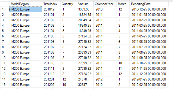
We will use only the first four columns, which are ModelRegion, TimeIndex, Quantity and Amount.
As discussed in the first article, create a sample analysis service project with Visual Studio or SQL Server Data Tools (SSDT). Then, create a Data Source connection to the AdventureWorksDW2017 database and add the vTimeSeries view to the Data Source View.
Next, create a Mining Structure with the Microsoft Time Series data mining technique. Select it from the available list of data mining techniques.
Then, select the necessary attributes to create the Time Series model. The Time Series model needs two compulsory parameters and one optional parameter. It requires a single time column which will be the key for the model. This has to be a column with the same intervals. For example, if you have monthly data, the entire data set should be monthly and should not contain different intervals of data. Another compulsory column is the column that you want to predict from the Time Series technique. This should be a continuous and numerical variable such as sales, temperature, quantity, etc.
Optionally, you can define multiple series in a one-time series. For example, in a sales time series, you might want to analyze the trend by region. Therefore, the region will be an additional and optional key.
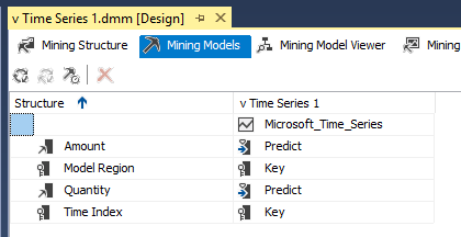
Here is the configuration for the parameters in the Time Series:
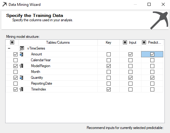
In the above configuration, both Quantity and Amount are configured as the input and prediction columns. As mentioned before, these two columns should be numerical and continuous variables. TimeIndex is the key column that is used to identify the time component of the data set. ModelRegion is the optional series column from which users can predict Region and Product Model quantities and sales amounts.
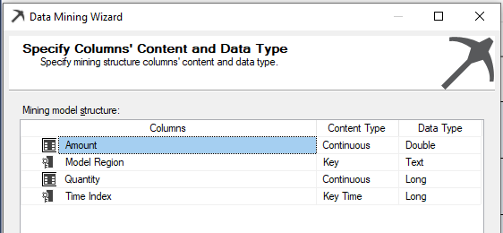
The following image shows data types, in case the user wants to change them:

However, in this example, you can leave the default data types as it is. With that, time series model creation is done, and the data mining model needs to be processed.
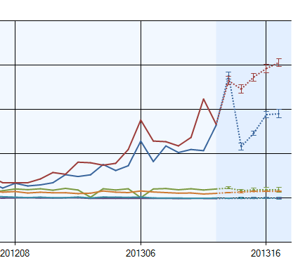
Let us view the time series trend with the predictions:
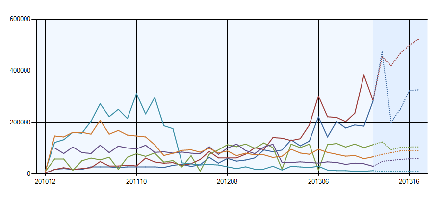
In the graph, predictions are shown by dotted lines. One important thing to remember is that the time series does not understand time index cycles. It just uses the number that follows the previous one. For example, after 201212, the next number will be 201213, not the calendar designation 201301.
From the configuration available at the top of the Mining Model Viewer, the user has the option to see more information.
By setting the Show Deviation to on, you can view the deviations for the predicted values to judge the accuracy of your model. A lower deviation means higher accuracy. Deviations are shown in the following image:
In the Mining Models tab, you can set the predictive attributes for Predict or PredictOnly as shown below:
Predict means the attribute is used to predict, and predicted value is used to predict the next values, whereas the PredictOnly parameter means the attribute is used only for prediction, and predicted value is not used for the next predictions.
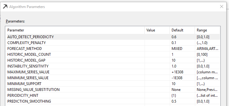
Model parameters
Model parameters are used to change the parameters to suit the data environment. Although the default parameters provide the best results, users have the option to change them accordingly:
AUTO_DETECT_PERIODICTY
This parameter specifies a value between 0 and 1 used to detect periodicity for the time series. By setting it to 1, the time series algorithm will automatically detect the periodicity. However, this can cause a performance issue during model building. Setting the value to 0 indicates that the algorithm will detect only the strong periodic data.
FORECAST_METHOD
FORECAST_METHOD specifies which forecasting algorithm is used. If the MIXED method is chosen, it creates models for both ARTXP and ARIMA time series algorithms, and their results will be combined during the prediction phase. In the standard edition of SQL Server, the models are combined using an automatic ratio that favors ARTXP for near-term and ARIMA for long-term prediction. In higher editions such as Enterprise edition, the models are combined and weighted according to the value set for PREDICTION_SMOOTHING. When the FORECAST_METHOD is set to either ARTXP or ARIMA, the value for the PREDICTION_SMOOTHING parameter is ignored.
PERIODICITY_HINT
This parameter provides a hint to the algorithm as to the periodicity of the data so the Time Series model performs better. Although the Time Series has the option of identifying the periodicity, it is better to provide the periodicity to the model. For example, if you have data with a periodicity of monthly, weekly and daily, you can configure PERODICITY_HINT such as {12,7,1}.
MISSING_VALUE_SUBSTITUTION
For Time Series, there cannot be gaps in the data set. However, due to various practical reasons, there may be instances where all data cannot be captured. SQL Server Time Series provides a method to substitute missing values. The default is None, which is suited for a data set without missing values. Mean values set the mean of the existing values to the missing values, whereas the Previous option sets the missing value with the previous values. Also, the user can set a constant value; this is not recommended.
Table of contents

View all posts by Dinesh Asanka
- Testing Type 2 Slowly Changing Dimensions in a Data Warehouse - May 30, 2022
- Incremental Data Extraction for ETL using Database Snapshots - January 10, 2022
- Use Replication to improve the ETL process in SQL Server - November 4, 2021