

Microsoft Clustering is the next data mining topic we will be discussing in our SQL Server Data mining techniques series. Until now, we have discussed a few data mining techniques like: Naïve Bayes, Decision Trees, Time Series, and Association Rules.
Microsoft Clustering is an unsupervised learning technique. In supervised training, there will be a variable that is already tagged to. In unsupervised training, there is no previously set variable as such.
Clustering is used to find out imperceptible natural grouping in a data set. This data set can be a large data set. Further, if there are a large number of attributes, you need a special technique to find natural grouping as the manual grouping is impossible.
Let us see how we can perform clustering in the Microsoft SQL Server platform. In this example, we will be using the vTargetMail view in the AdventureWorksDW sample database, as we did for previous examples in the series.
Let us first create a data source and the Data Source View as we did in the other examples. In this, the data source would be AdventureWorksDW, while vTargetMail is the data source views.
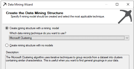
In the wizard, the next is to choose the data mining technique:
Since there is only one view in the Data Source View, vTargetMail will be the Case table and next is to choose relevant attributes as shown in the below screenshot:
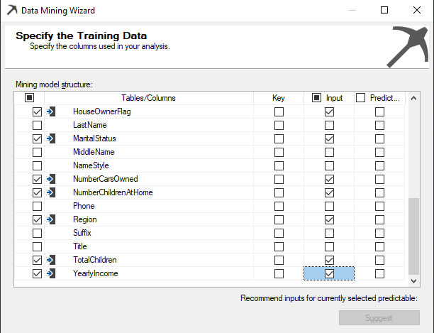
In the above, the Customer Key is chosen as the Key from the algorithm. Since it is assumed that attributes such as Middle Name, Title will not make major contributions towards the natural grouping, input variables are chosen with sense. If not, there will be unnecessary processing time for the data mining structures. So in the above selection, Age, BikeBuyer, CommuteDistance, EnglishEducation, EnglishOccupation, Gender, HouseOwnerFlag, MaritalStatus, NumberCarsOwned, NumberChildrenatHome, Region, TotalChildren and YearlyIncome were chosen as relevant attributes.
Since we are using the Microsoft Clustering algorithm, there is no need to choose Predict variable. This is why we said earlier that the Microsoft Clustering is an unsupervised learning technique.
Next is to select the correct Content types, though there are default Content types. Content types can be modified from the following screen:
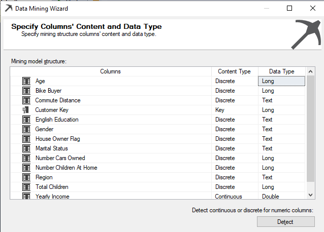
In the above screenshot, for the numerical data type or long data type, the default content type will be Continuous. For example, columns like Age, Number Cars owned are numeric data types. Though they are numeric, we know that values are Discrete as Number Cars Owned contain values such as 0, 1, 2, 3, etc. Content-Type of Age, Bike Buyer, Number Cars Owned, Number Children at Home and Total Children attributes were changed to Discrete from Continuous. We will leave the Yearly Income content type as Continuous.
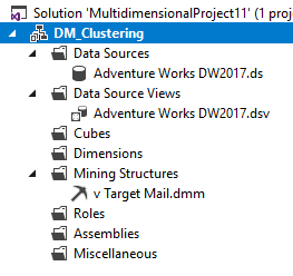
In the data mining wizard, default settings are used and now you are ready to process the data mining structure as shown in the below screenshot. This is the Solution Explorer for the Clustering data mining technique:
After processing the data mining structure, now let us view the results. There are four analysis graphs: Cluster Diagram, Cluster Profiles, Cluster Characteristics, and Cluster Discrimination.
Cluster Diagram
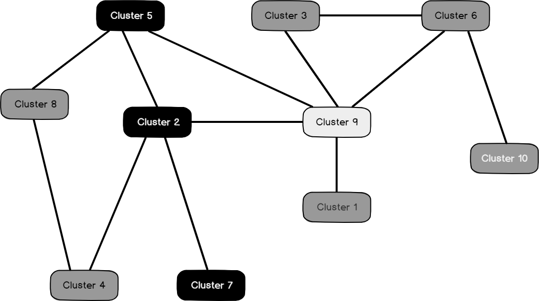
The cluster diagram has main two features. You can find the cluster distribution from the Cluster diagram. From the available drop-down, you can find the relevant cluster. When the relevant values are selected, the color will change accordingly.
Following is the Cluster diagram for Bike buyer =1. This means Cluster 5, Cluster 9 and Cluster 4 have the Bike buyer = 1:

Following is the Cluster diagram for Marital Status = S:
You can select the attribute and its values from the two available dropdowns.
In addition, a Cluster diagram can find out similar clusters and weak and strong links by moving the sliders up or down.
Cluster Profiles
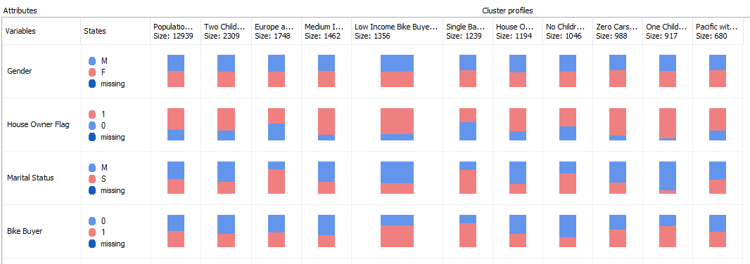
Each cluster has its own property. You can view the cluster profiles from this view. Since there are a few numbers of attributes, cluster profiles are shown in two images.
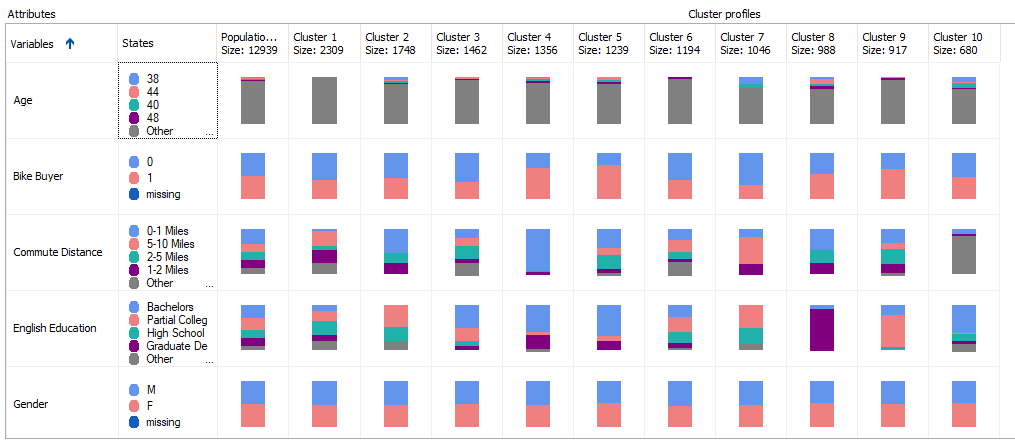
This is the first screenshot, which shows Age, Bike Buyer, Commute Distance, English Education, and Gender attributes:
This is the second screenshot, which shows Number Children at Home, Region, Total Children, Yearly Income attributes:
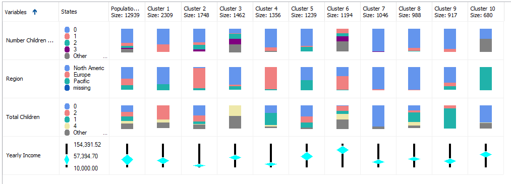
Except for Yearly Income, all the other attributes are dropdowns attributes that are shown in stack bars. Continuous attribute, Yearly Income is shown as five numbers (Minimum, Maximum, Mean, First Quartile, and Third Quartile) format.
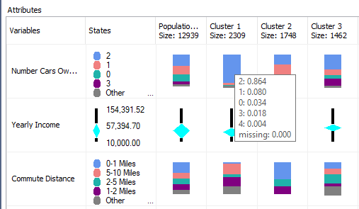
If you make a move on top of each stack, you will see the contributions, as shown in the below screenshot:
If you closely look at these cluster profiles, you will see that Cluster 4, Cluster 5 and Cluster 9 have a higher percentage of Bike Buyers. Out of those three clusters, Cluster 4 has the highest percentage of customers who do not have a car. Further, you will see that Cluster 4 is a Low-Income as well. This means Cluster 4 can be labeled as Low Income Bike Buyers without a Car. You can rename the cluster with a business-friendly name accordingly that is shown in the below image:
After naming these clusters, if you go back to the previous cluster diagram, you will see that new cluster names are updated, as shown in the below screenshot:
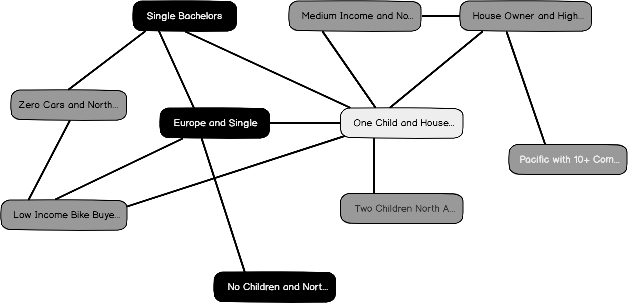
With this rename option, your cluster profiles are much readable than using the default cluster names.
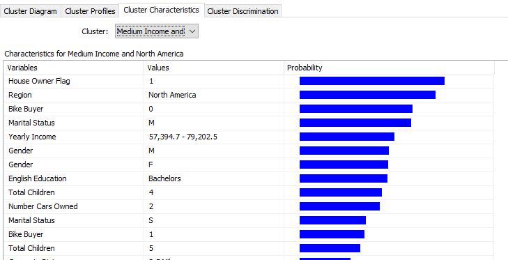
Cluster Characteristics
You can view the characteristics of clusters using the Cluster Characteristics tab, as shown in the below screenshot:
Cluster Discrimination
Since there are ten clusters in this example, sometimes you might be interested to know the difference between the two clusters. By choosing any two clusters, you will understand the difference between the selected clustered, as shown in the below screenshot:
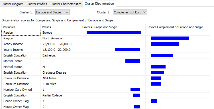
In the above screenshot, the first cluster predominantly has customers in Europe while the other cluster contains customers from North America.
Algorithm Parameters
As we discussed in the previous articles, we can gain better results by modifying the algorithm parameters from the following screenshot:
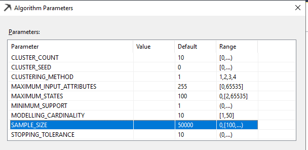
Let us look at important parameters for the Microsoft Clustering technique.
Cluster Count
This parameter defines the number of clusters. As you can remember, we had 10 clusters in the example. There is no limit on the number of clusters. If this value is set to 0, a number of clusters will be decided by the algorithm. However, it is essential to limit the number of clusters to visualize better results and of course, the performance of the model. Typically, cluster count 5 is the optimal value.
Cluster Method
The clustering method algorithm uses can be:
- Scalable EM
- Non-scalable EM
- Scalable K-means
- Non-scalable K-means
In Microsoft Clustering, there are two main methods for clustering: Expectation-Maximization (EM) and K-Means. EM cluster assignment method uses a probabilistic measure while K-Means uses Euclidean distance. EM method is also called as soft clustering as one object can be fallen into multiple clusters with different probabilities. Conversely, the K-mean clustering is called Hard Clustering.
Clustering is an iterative process. If there are a large number of data points, a large amount of memory will be consumed. With the scalable framework, if the algorithm finds that the data point is not going to change its cluster, those points are removed from the iteration. In this technique, data is loaded by chunk. The number of data points is defined by the SAMPLE SIZE parameter. By doing so, the clustering technique will be much scalable.
Sample Size
If you have chosen any scalable clustering option, this parameter defines how many data points should be selected for each iteration. The default value is 50,000.
Stopping Tolerance
This parameter determines the convergence point for the iteration process to stop. Increasing this number will cause the iteration to stop quickly. If you have a large data set, you can increase this value.
Cluster Prediction
The next important aspect is predicting the cluster for a given data set. This can be done by using the Mining Model prediction tab.
First, you need to select the built data mining model. We will check the cluster for a one value set; hence we should select, Singleton Query option from the top:
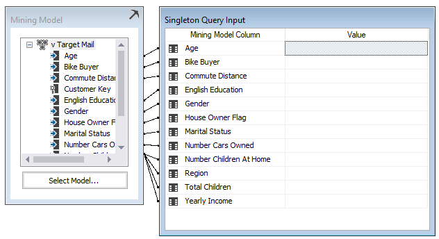
Now we need to enter values for each attribute. For the nominal variables, you need to select from the available values, whereas, for the continuous variables like Yearly Income, you need to type a value.
The following screenshot shows how values are entered for a variable:
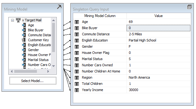
In case you don’t know values for any variables, you can tag that as Missing. However, it is important to catch as much as values possible.
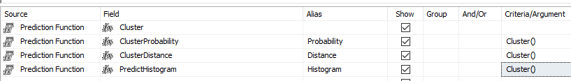
Then you will choose Prediction function in the bottom half of the screen, as shown below:
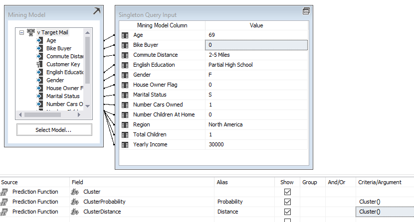
When the result option is clicked, you will get the following results, showing the relevant cluster that this data set belongs to:
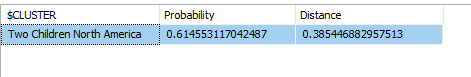
This result indicates that your data set belongs to the Two Children North America cluster with 0.61 probability. The Distance parameter indicates how far your data set is from this cluster. Basically, it is the inverse of the probability.
Then your next question would be what other probable clusters are. This can be obtained from the Predication function, Histogram, as shown in the below screenshot:
The following screenshot shows the results for the above prediction function:
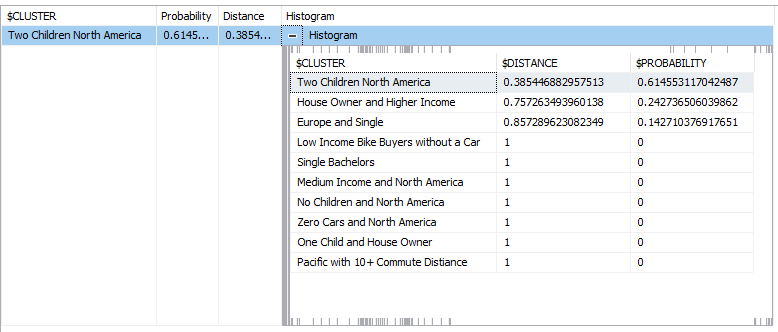
The above result shows that this particular data set belongs to three different clusters with different probabilities.
Summary
Clustering is an unsupervised technique that can be used to create natural grouping in a data set. There are two main techniques K-Means and EM. To facilitate large data volumes, the scalable option is available too. In Microsoft Clustering, there are multiple views to get more details into the clustering. Cluster Diagram provides you with the relationship of available clusters. The cluster Profile view provides the pictorial view of the cluster profiles. The Cluster Characteristics view will provide you with the details of a selected cluster, whereas Cluster Discrimination will provide you the option of comparison of two selected clusters.
From the built model, predications can be done where we can get the cluster it belongs to and its probability.
Table of contents

View all posts by Dinesh Asanka
- Testing Type 2 Slowly Changing Dimensions in a Data Warehouse - May 30, 2022
- Incremental Data Extraction for ETL using Database Snapshots - January 10, 2022
- Use Replication to improve the ETL process in SQL Server - November 4, 2021