
Introduction
In past chats, we have had a look at a myriad of different Business Intelligence techniques that one can utilize to turn data into information. In today’s get together we are going to have a look at a technique dear to my heart and often overlooked. We are going to be looking at data mining with SQL Server, from soup to nuts.
Microsoft has come up with a fantastic set of data mining tools which are often underutilized by Business Intelligence folks, not because they are of poor quality but rather because not many folks know of their existence OR due to the fact that people have never had to opportunity to get to utilize them.
Rest assured that you are NOW going to get a bird’s eye view of the power of the mining algorithms in our ‘fire-side’ chat today.
As I wish to describe the “getting started” process in detail, this article has been split into two parts. The first describes exactly this (getting started), whilst the second part will discuss turning the data into real information.
So ‘grab a pick and shovel’ and let us get to it!
Getting started
For today’s exercise, we start by having a quick look at our source data. It is a simple relational table within the SQLShackFinancial database that we have utilized in past exercises.
As a disclosure, I have changed the names and addresses of the true customers for the “production data” that we shall be utilizing. The names and addresses of the folks that we shall utilize come from the Microsoft Contoso database. Further, I have split the client data into two distinct tables: one containing customer numbers under 25000 and the other with customer numbers greater than 25000. The reason for doing so will become clear as we progress.
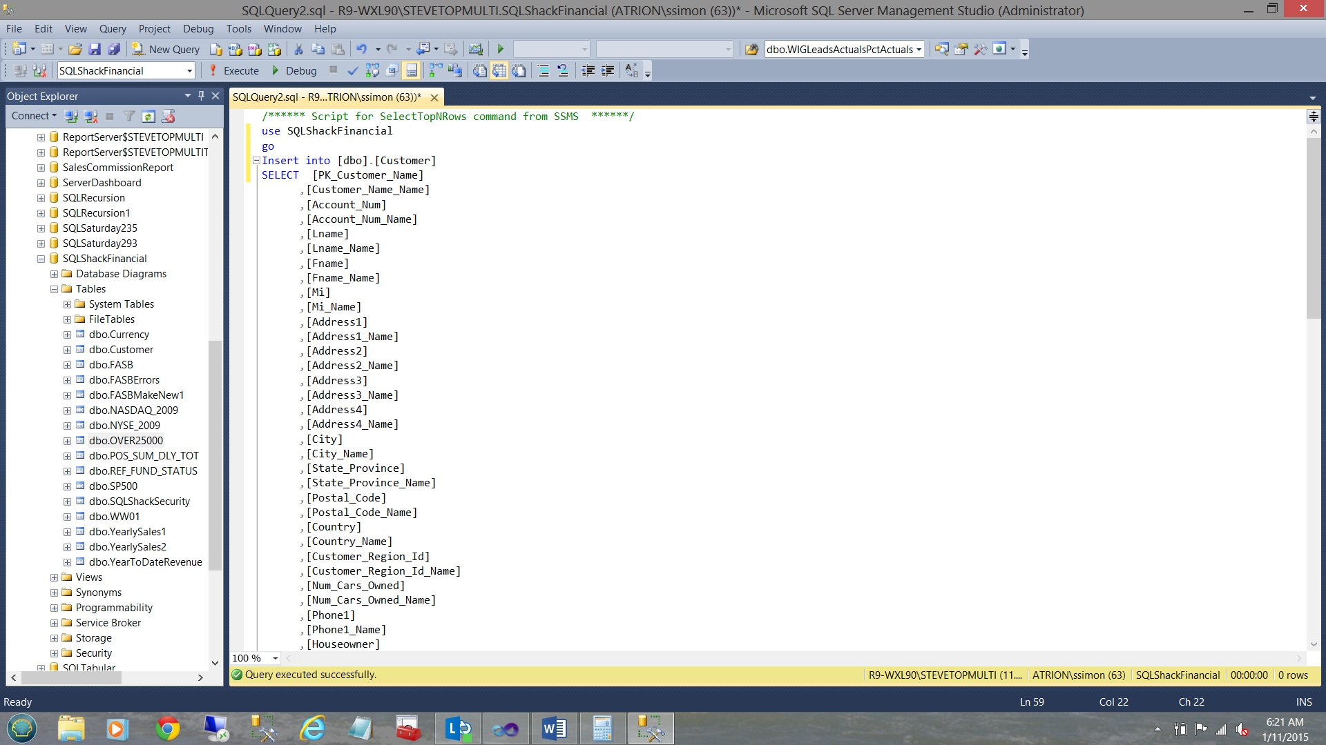
Having a quick look at the customer table (containing customer numbers less than 25000), we find the following data.
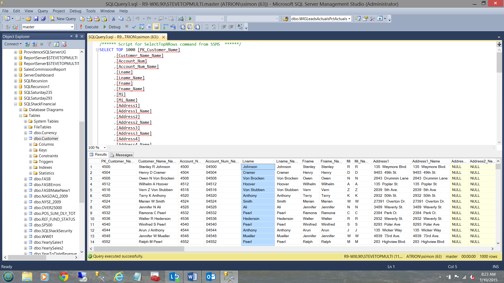
The screenshot above shows the residential addresses of people who have applied for financial loans from SQLShack Finance.
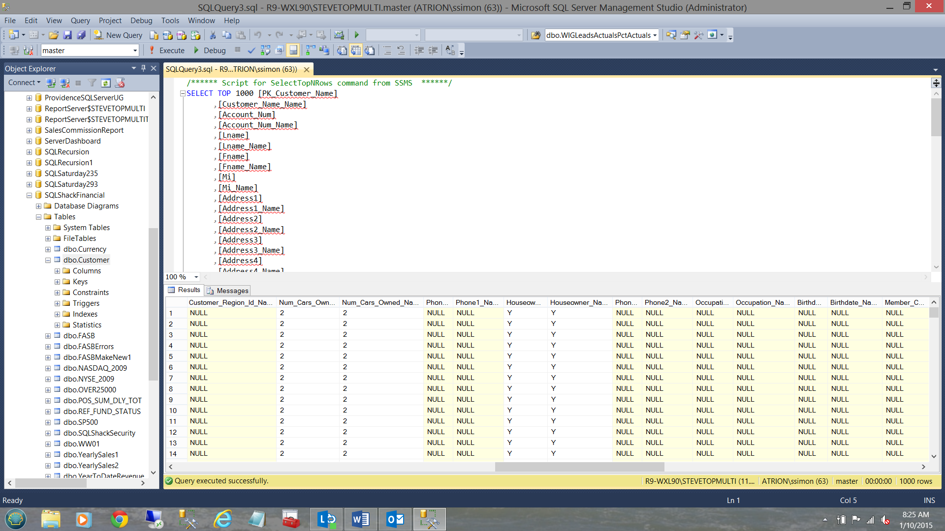
Moreover, the data shows criteria such as the number of cars that the applicant owns, his or her marital status and whether or not he or she owns a house. NOTE that I have not mentioned the person’s income or net worth. This is will come into play going forward.
Creating our mining project
Now that we have had a quick look at our raw data, we open SQL Server Data Tools (henceforward referred to as SSDT) to begin our adventure into the “wonderful world of data mining”.
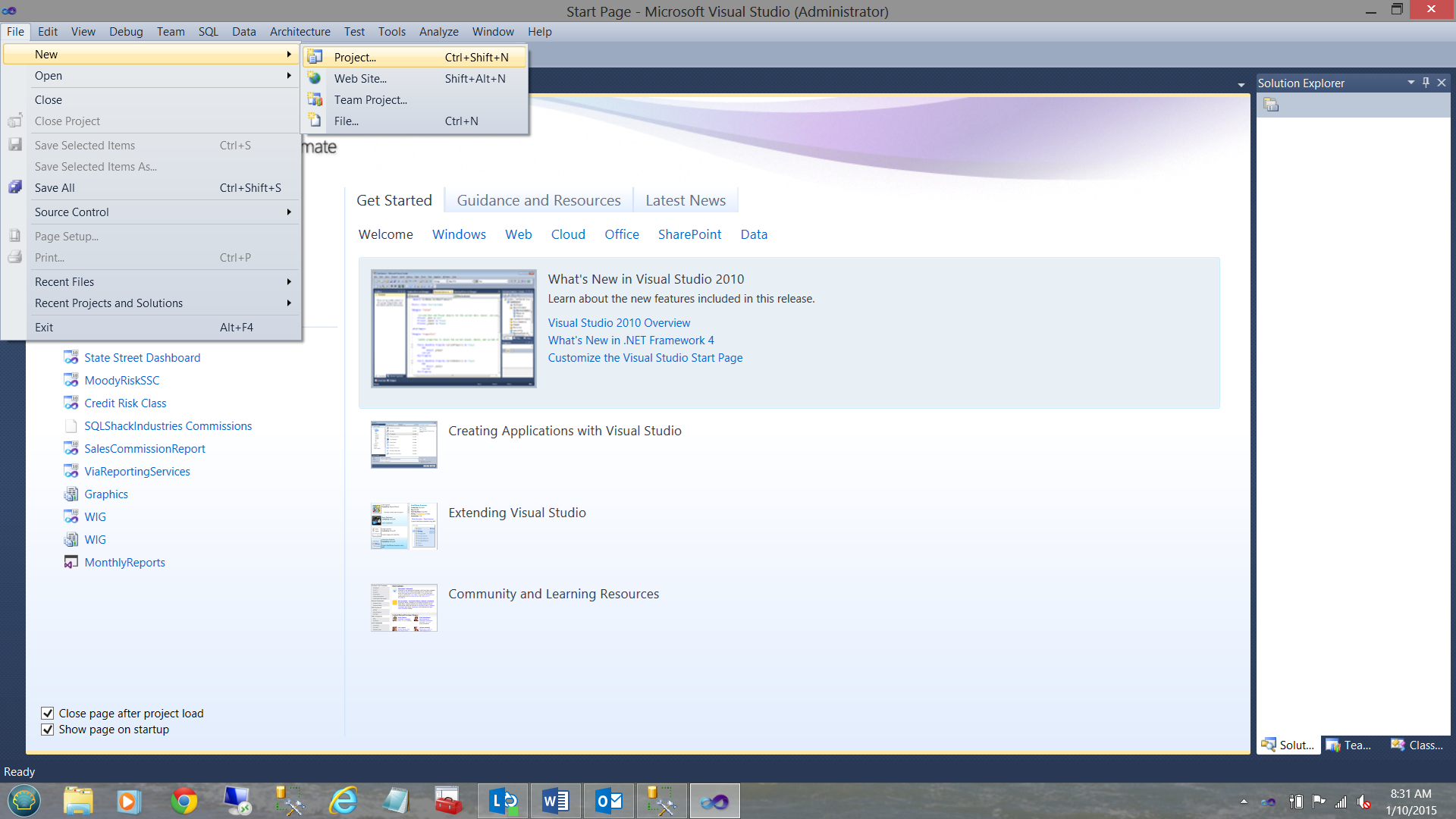
Opening SSDT, we select “New” from the “File” tab on the activity ribbon and select “Project” (see above).
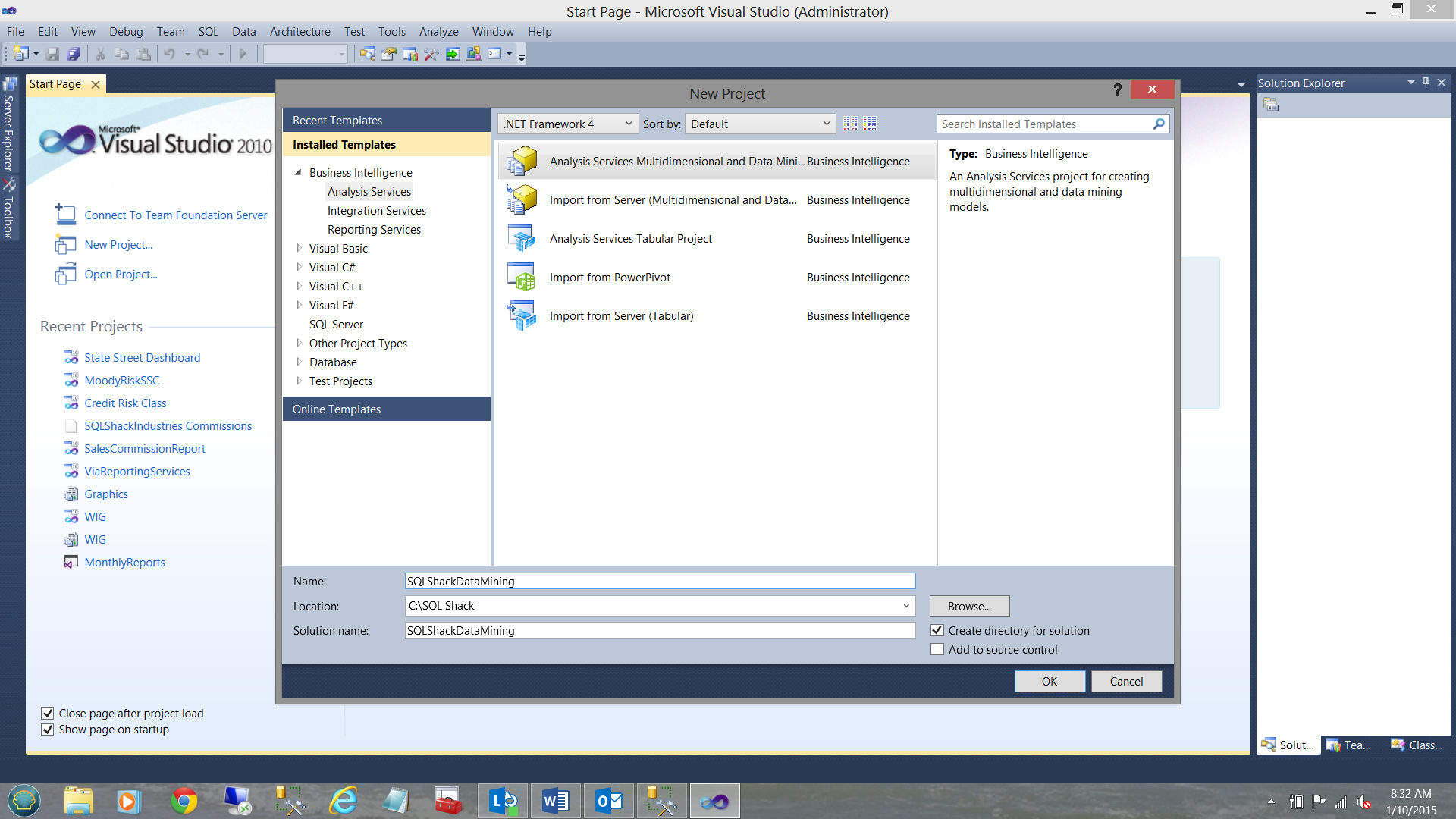
We select the “Analysis Services Multidimensional and Data Mining” option. We give our new project a name and click OK to continue.
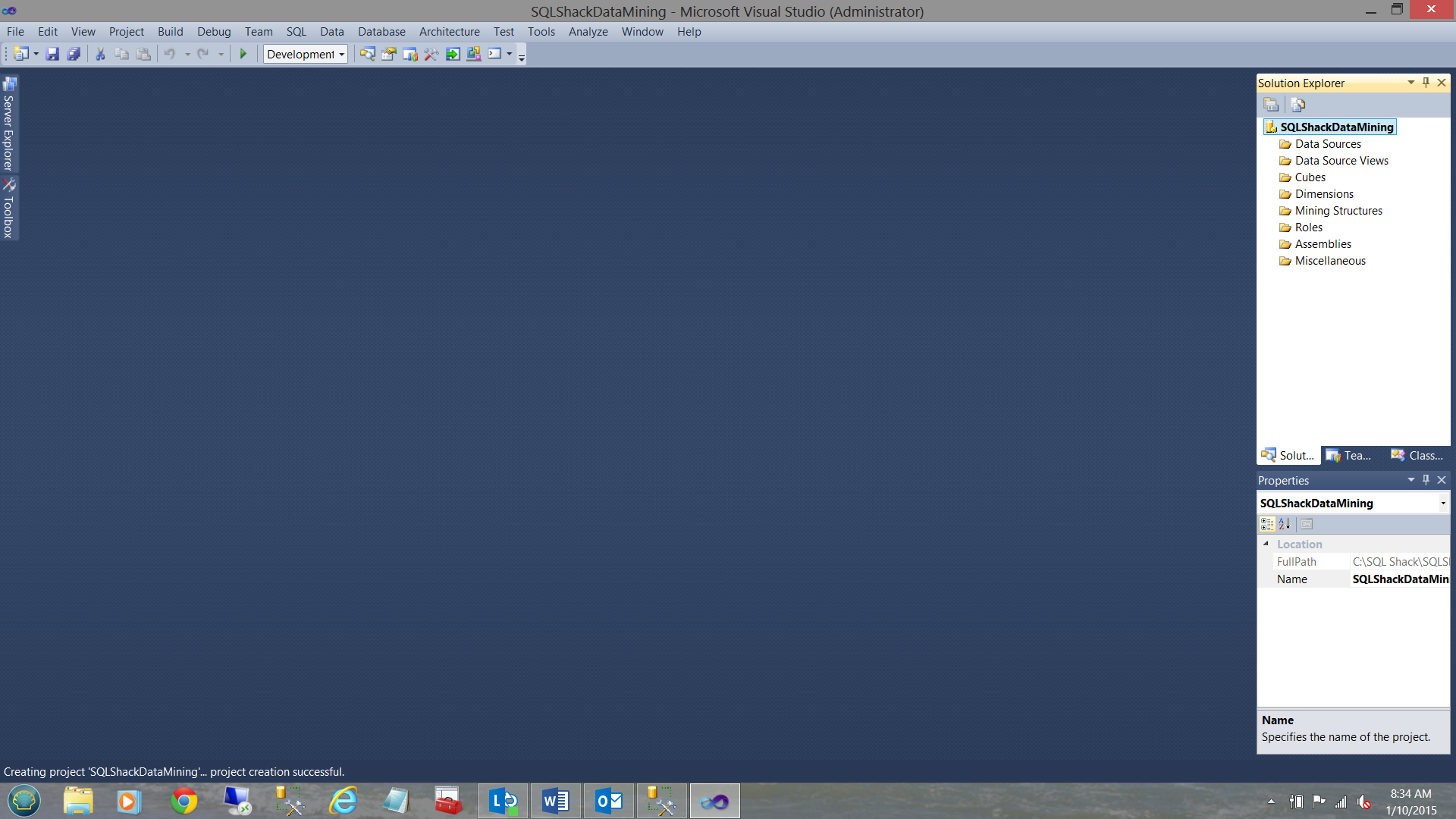
Having clicked “OK”, we find ourselves on our working surface.
Our first task is to establish a connection to our relational data. We do this by creating a new “Data Source” (see below).
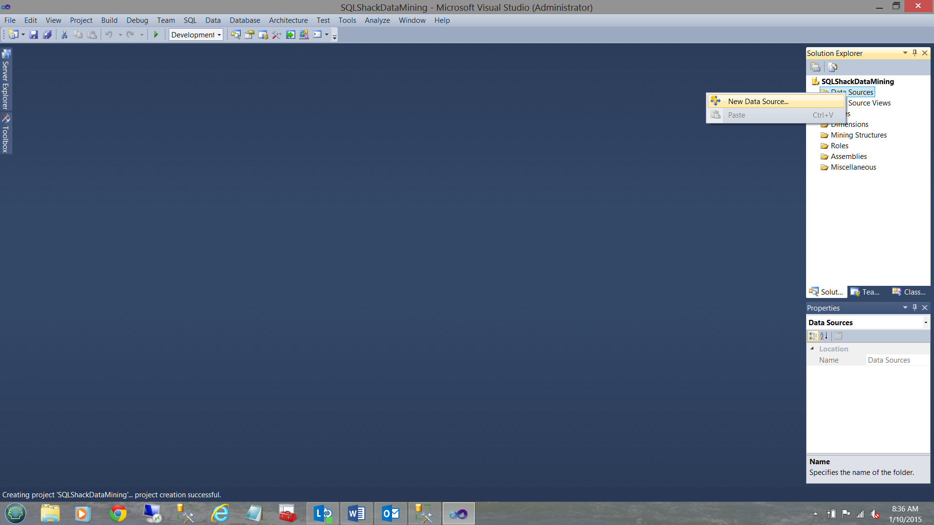
We right-click on the “Data Sources” folder (see above and to the right) and select the “New Data Source” option.
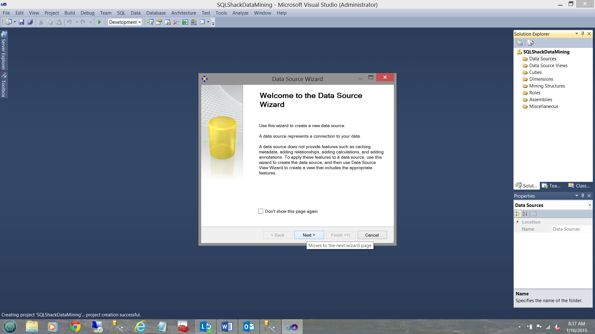
The “New Data Source” Wizard is brought up. We click “Next”.
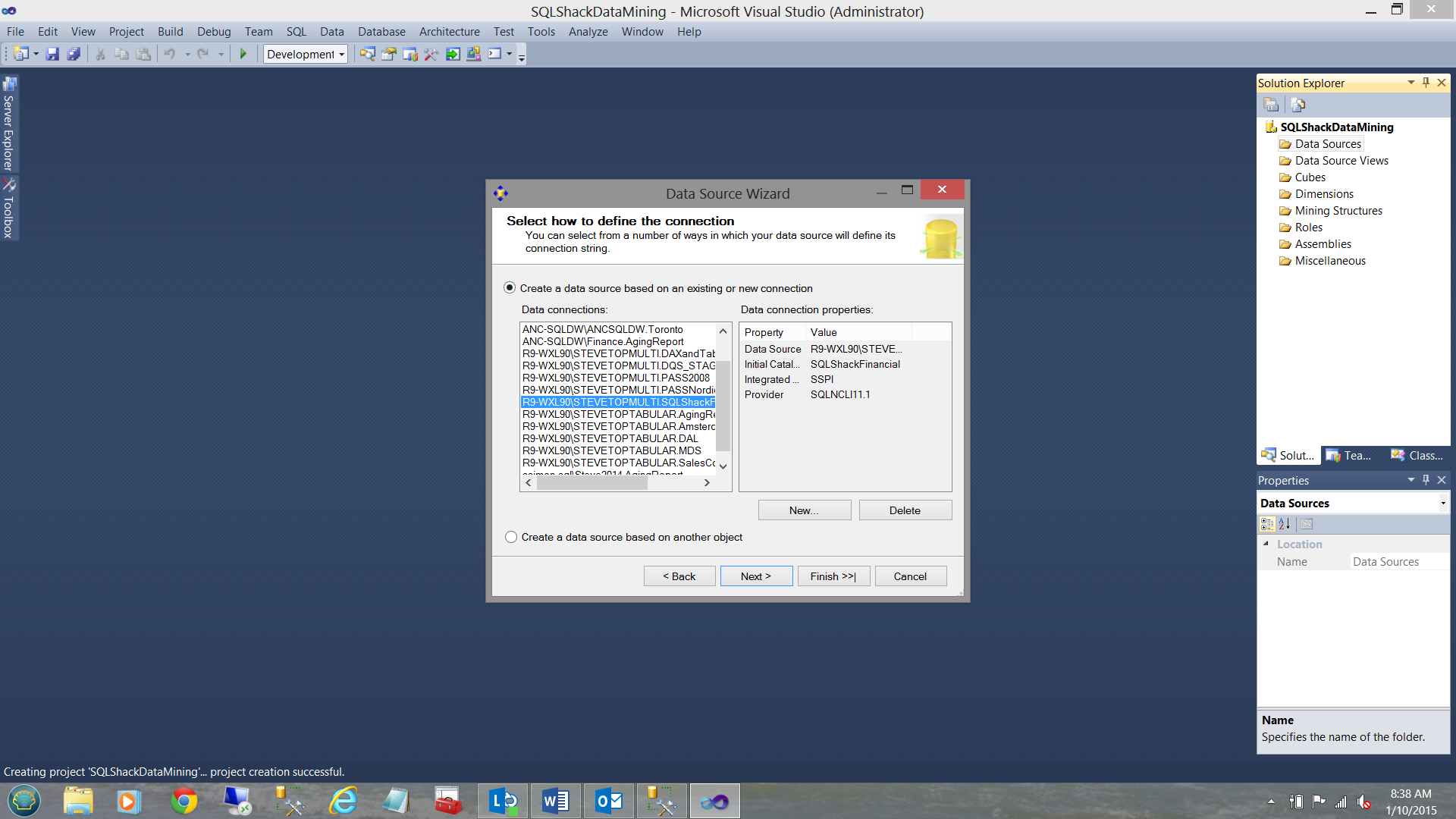
We now find ourselves looking at connections that we have used in past and SSDT wishes to know which (if any) of these connections we wish to utilize. We choose our “SQLShackFinancial” connection.
We select “Next”
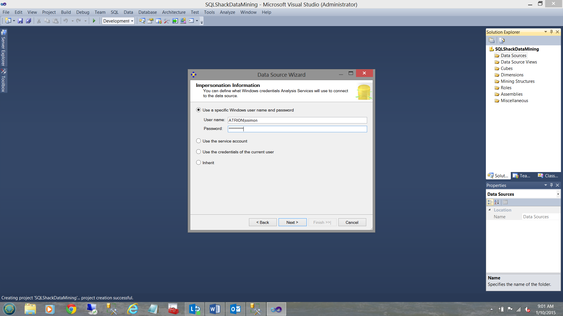
We are asked for our credentials (see above) and click next.
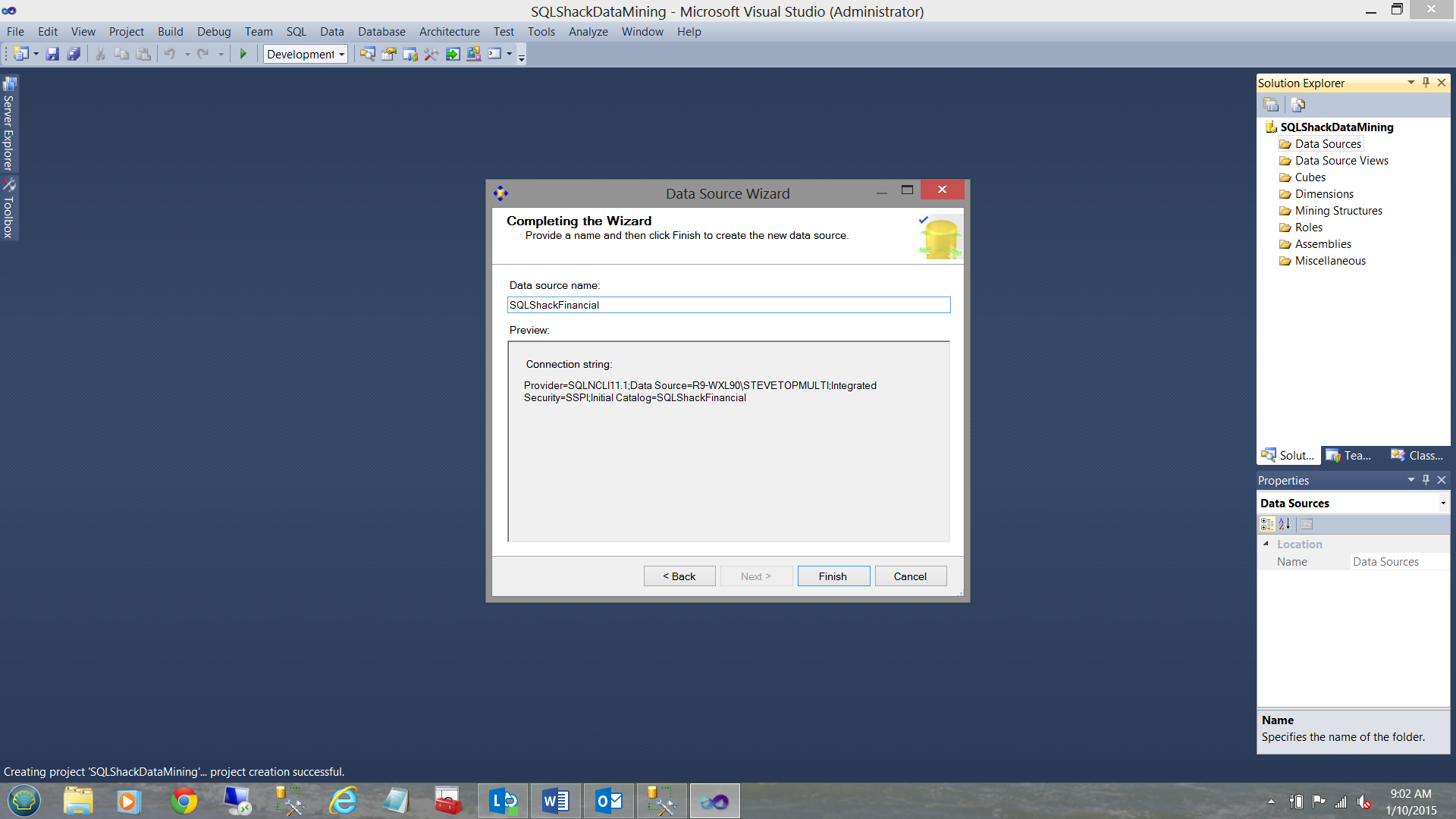
We are now asked to give a name to our connection (see above).
We click finish.
Creating our Data Source View
Our next task is to create a Data Source View. This is different to what we have done in past exercises.
The data source view permits us to create relationships (from our relational data) which we wish to carry forward into the ‘analytic world’. One may think of a “Data Source View” as a staging area for our relational data prior to its importation into our cubes and mining models.
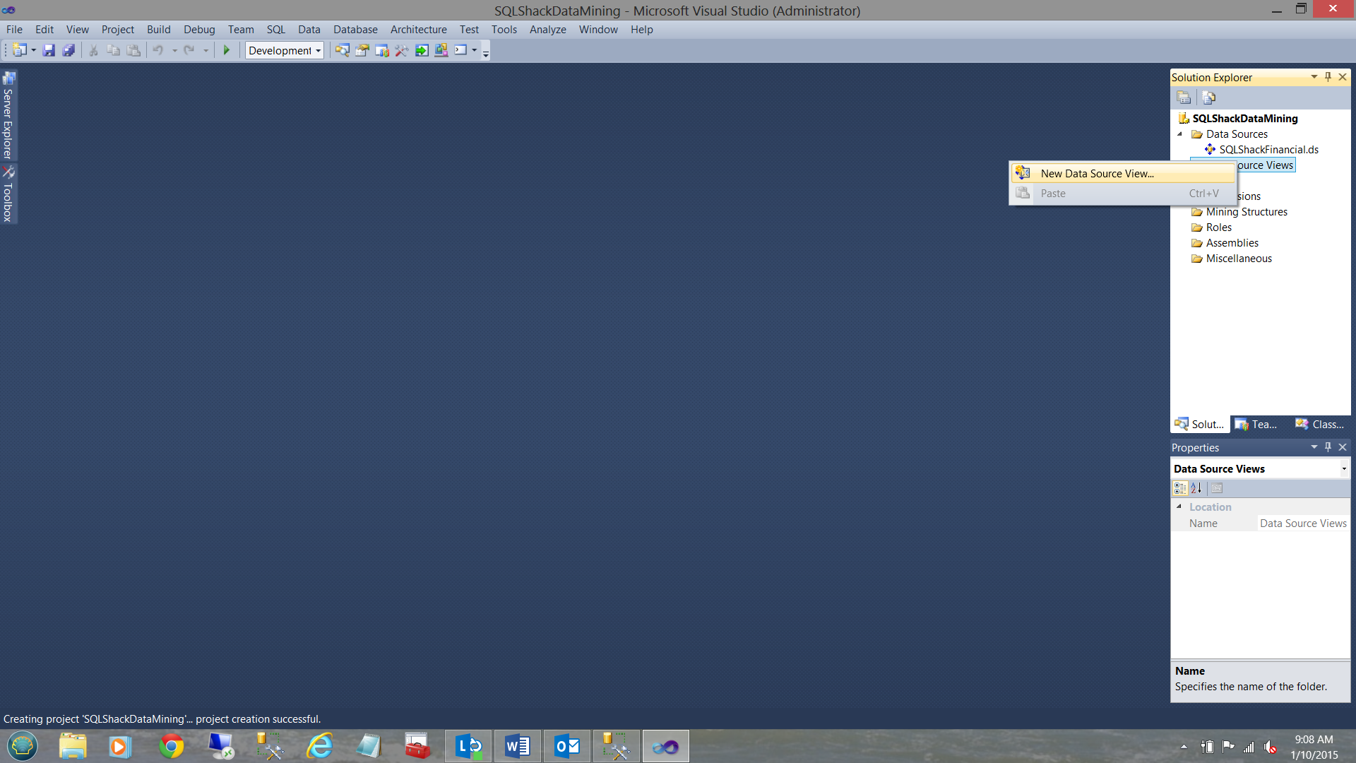
We right-click on the “Data Source Views” folder and select “New Data Source View”.
The “Data Source View” wizard is brought up (see below).
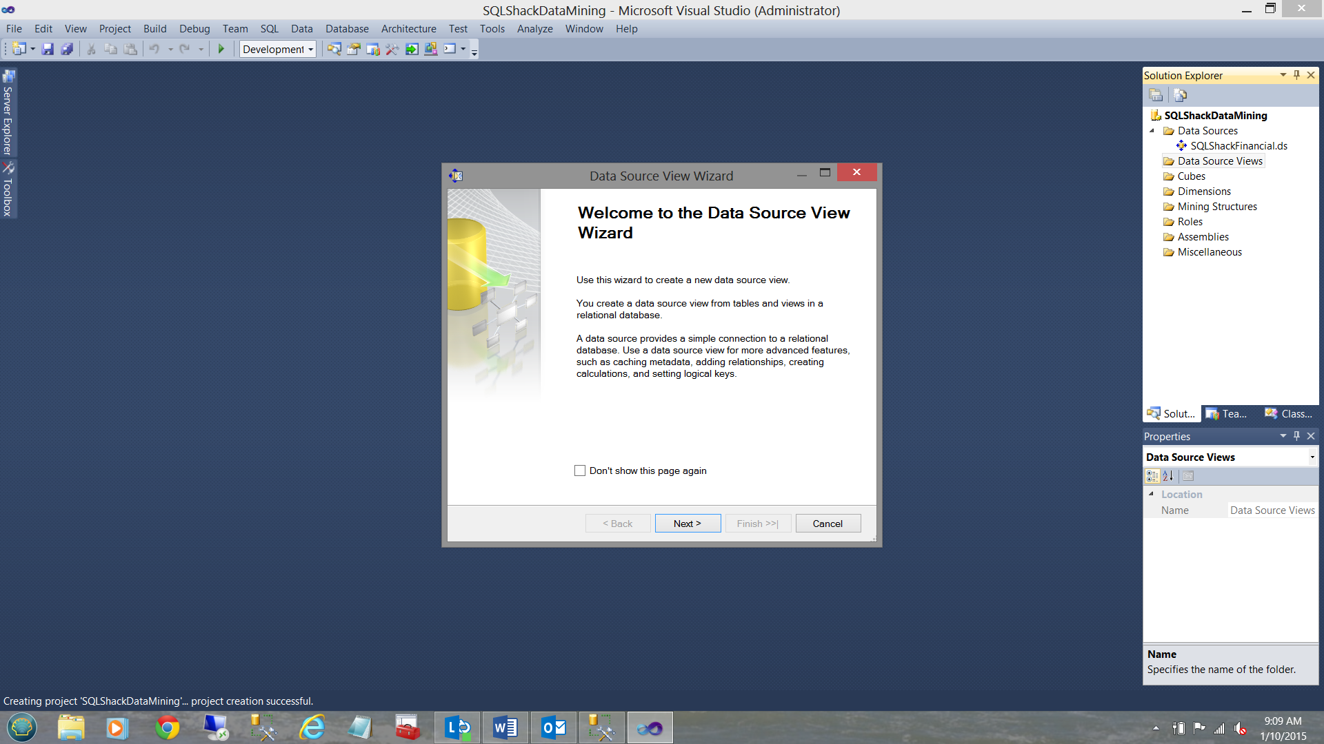
We click “Next” (see above).
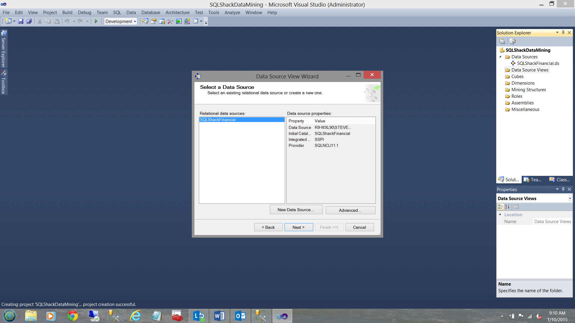
We select our “Data Source” that we defined above (see above).
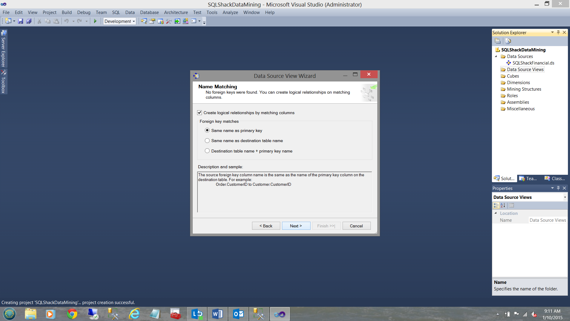
The “Name Matching” dialogue box is brought into view. As we shall be working with one table for this exercise, there is not much impact from this screen HOWEVER if we were creating a relationship between two or more tables we would indicate to the system that we want it to create the necessary logical relationships between the two or more tables to ensure that our tables are correctly joined.
In our case we merely select “Next” (see above).
We are now asked to select the table or tables that we wish to utilize.
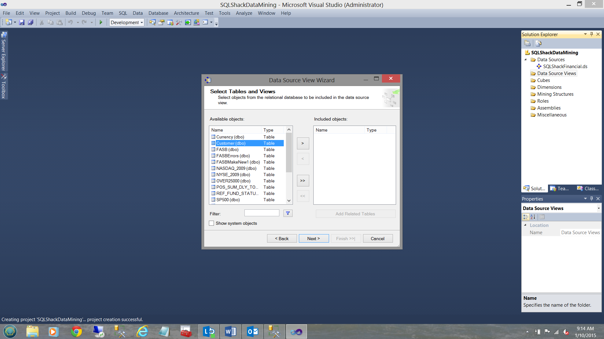
For our current exercise, I select the “Customer” table (See above) and move the table to the “Included Objects” (see below).
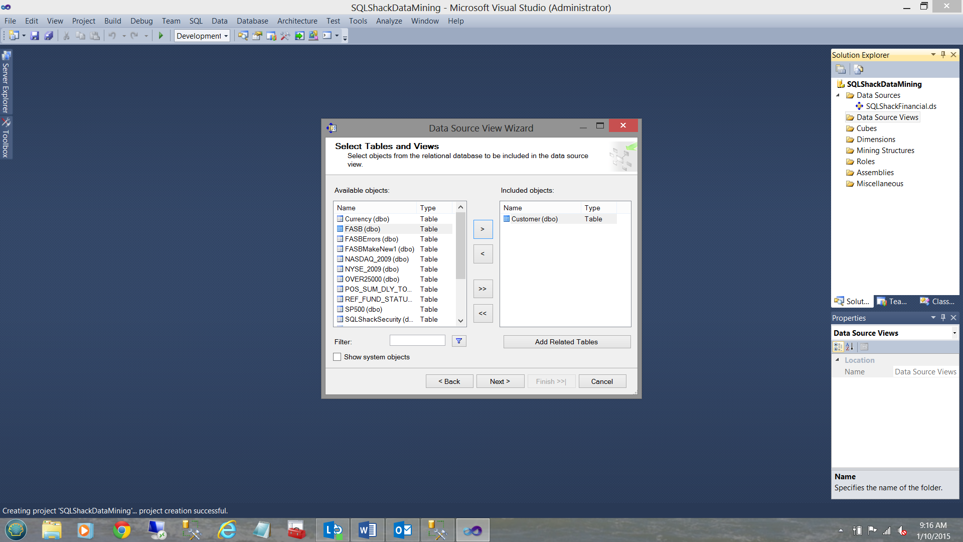
We then click “Next”.
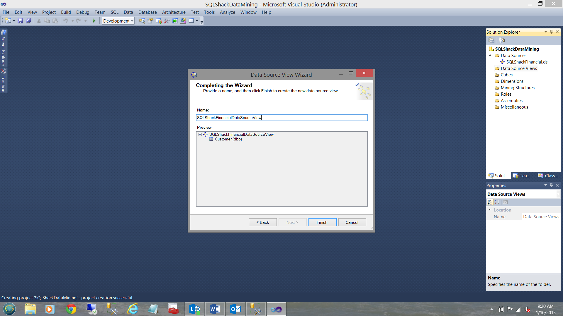
We are now asked to give our “Data Source View” a name (see above) and we then click “Finish” to complete this task.
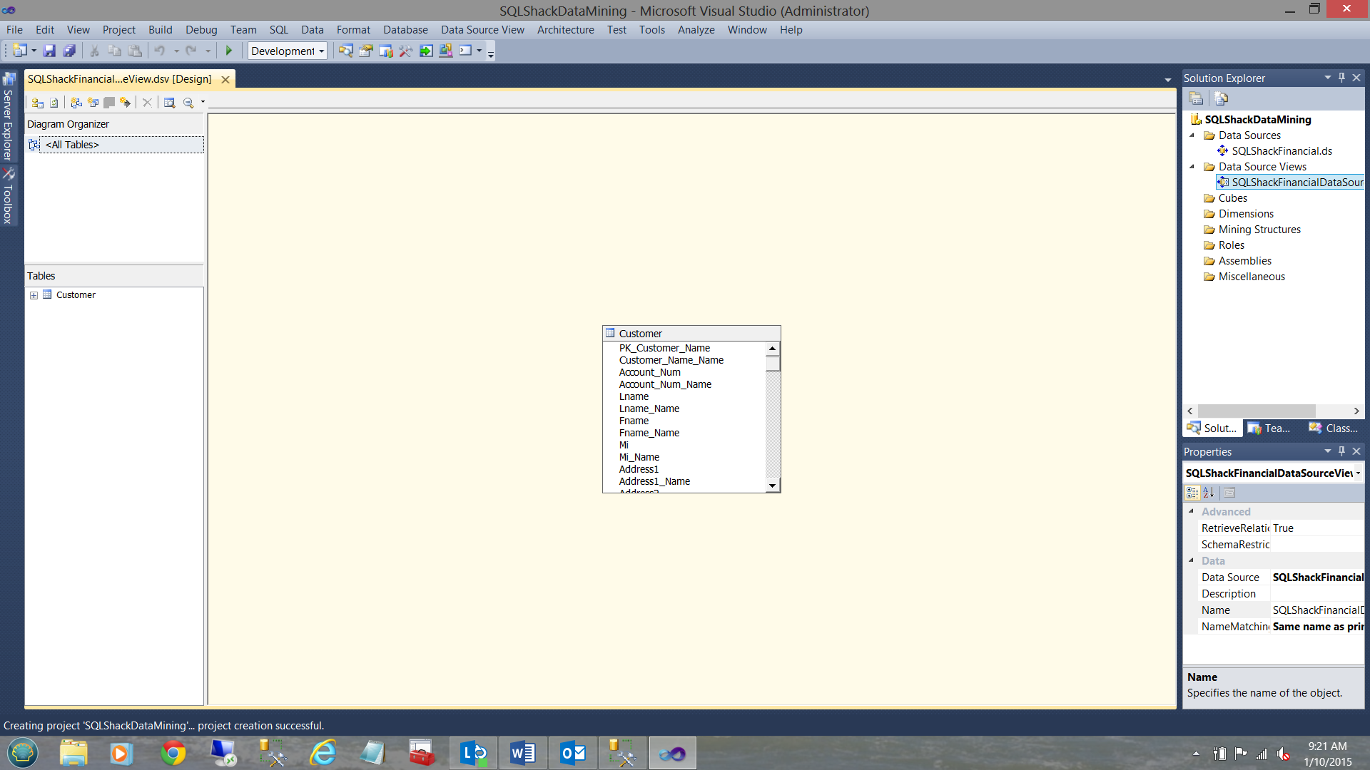
We find ourselves back on our work surface. Note that the Customer entity is now showing in the center of the screenshot above, as is the name of the “Data Source View” (see upper right).
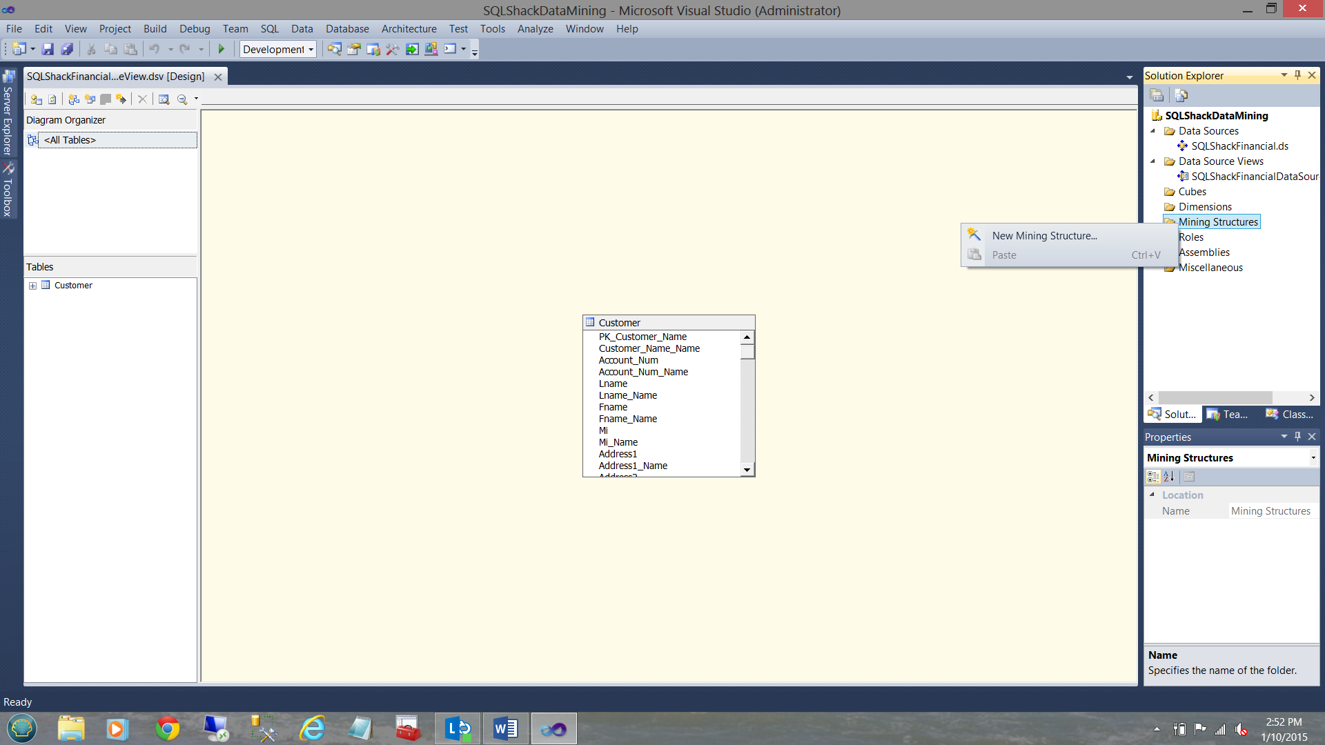
We now right click on the ‘Mining Structure” folder and select “New Mining Structure” (see above).
The “Data Mining Wizard” now appears (see below).
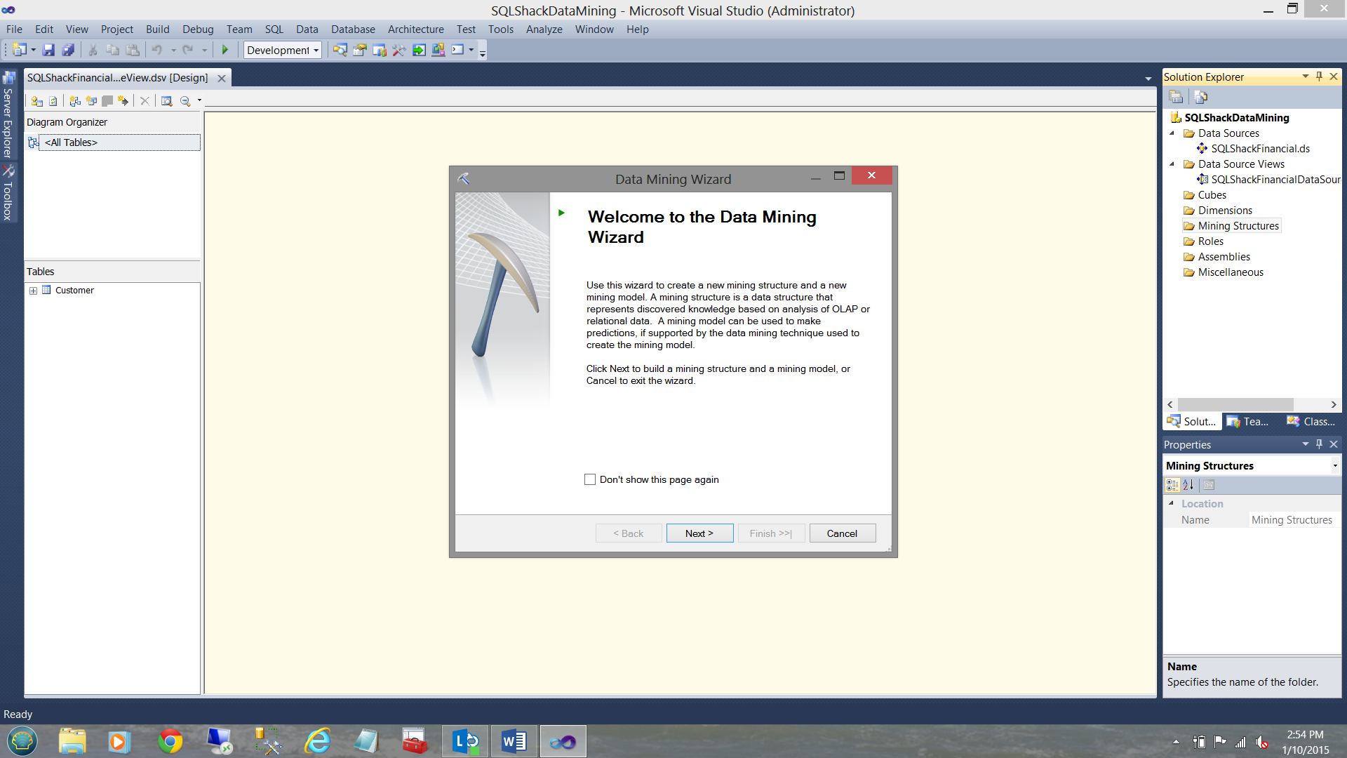
We click “Next”.
For the “Select the Definition Method” screen we shall accept the default “From existing relational database or data warehouse” option (see below).
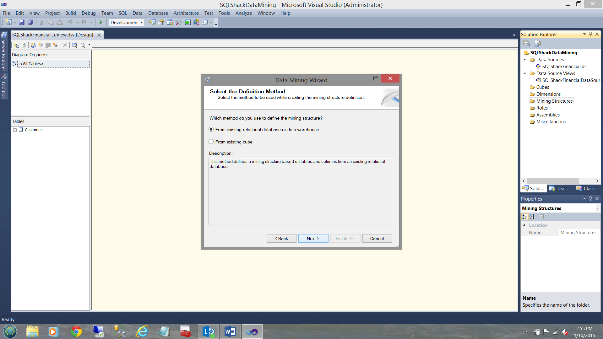
We then click “Next”.
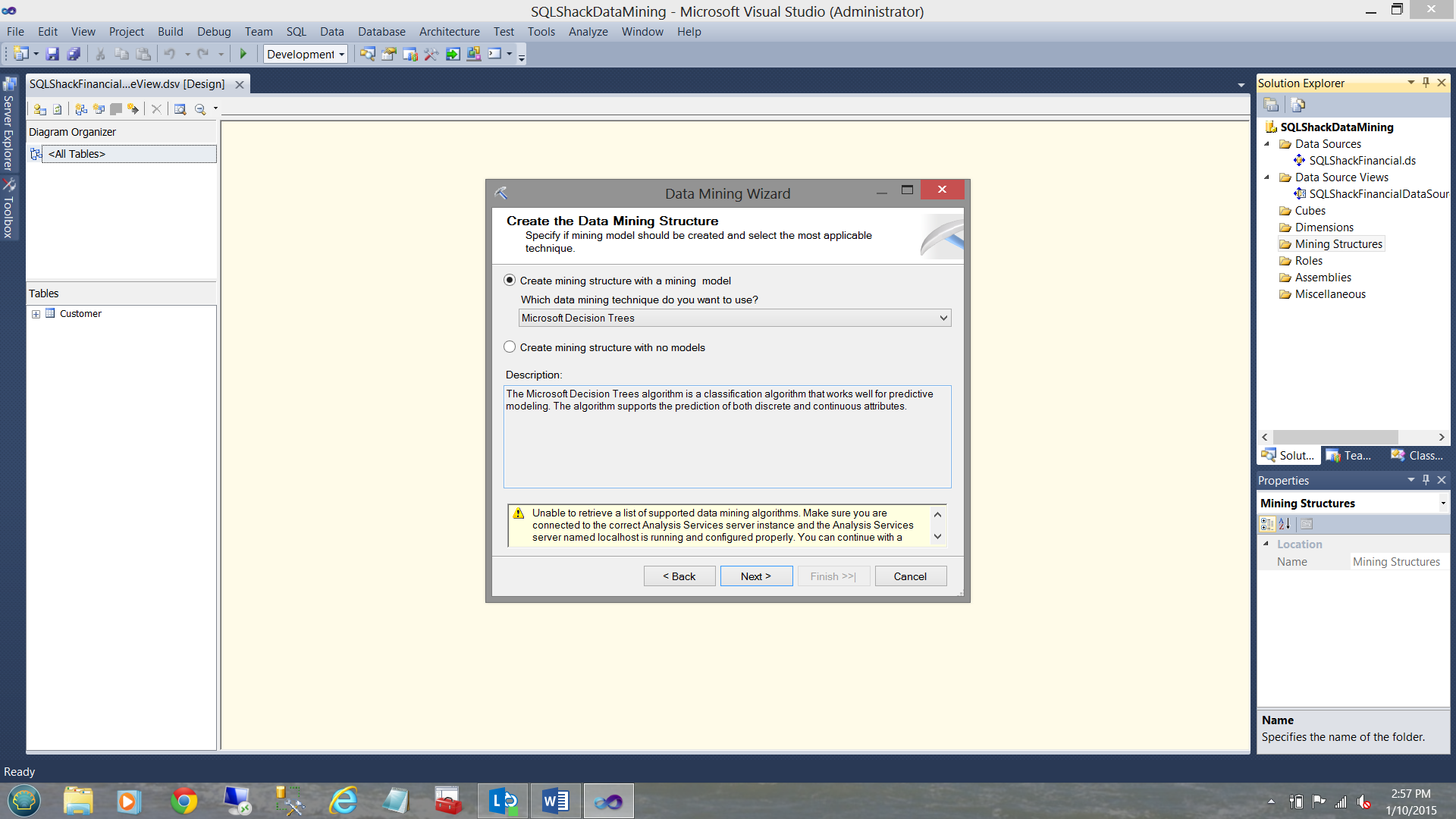
The “Create the Data Mining Structure” screen is brought into view. The wizard asks us which mining technique we wish to use. In total for this exercise, we shall be creating four structure. “Microsoft Decision Trees” is one of the four. That said, we shall leave the default setting “Microsoft Decision Trees” as is.
We ignore the warning shown in the message box as we shall create the necessary connectivity on the next few screens.
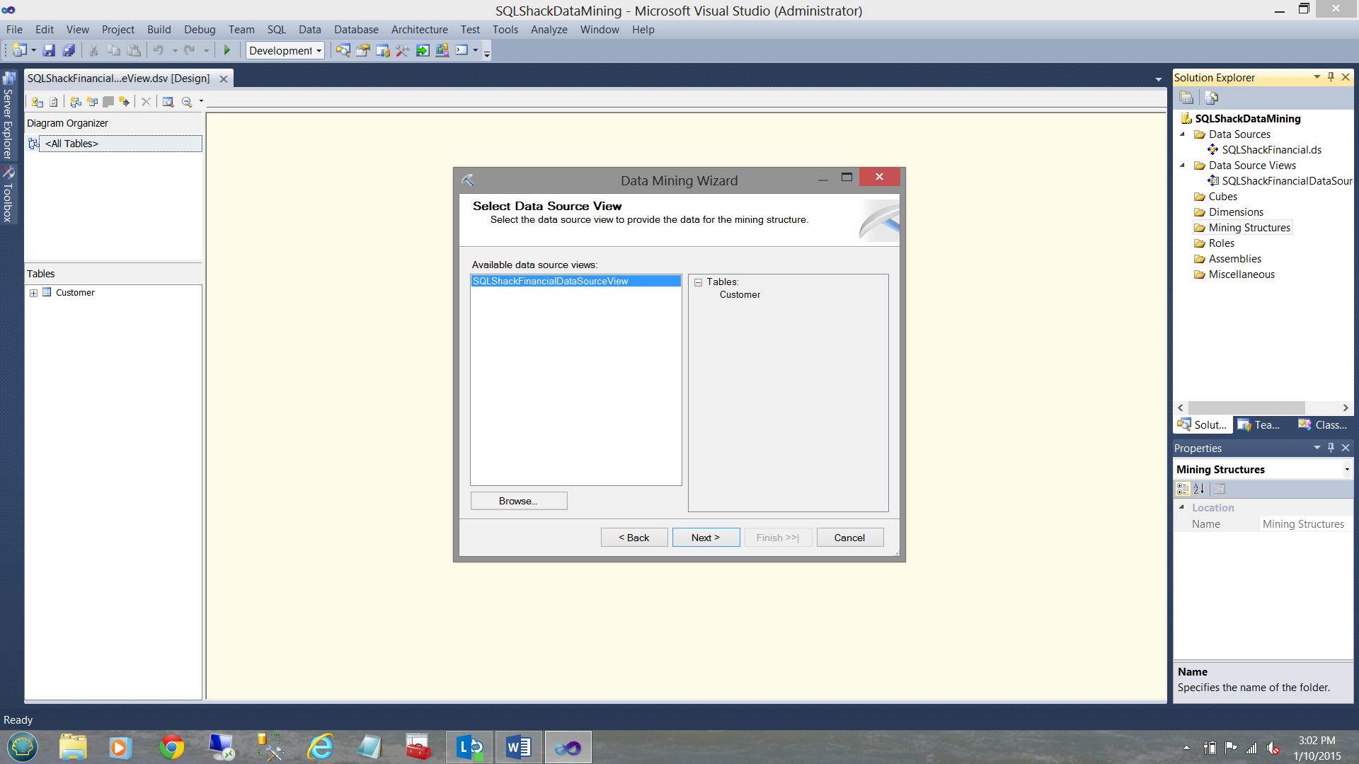
The reader will note that the system wishes to know which “Data Source View” we wish to utilize. We select the one that we created above. We then click “Next”.
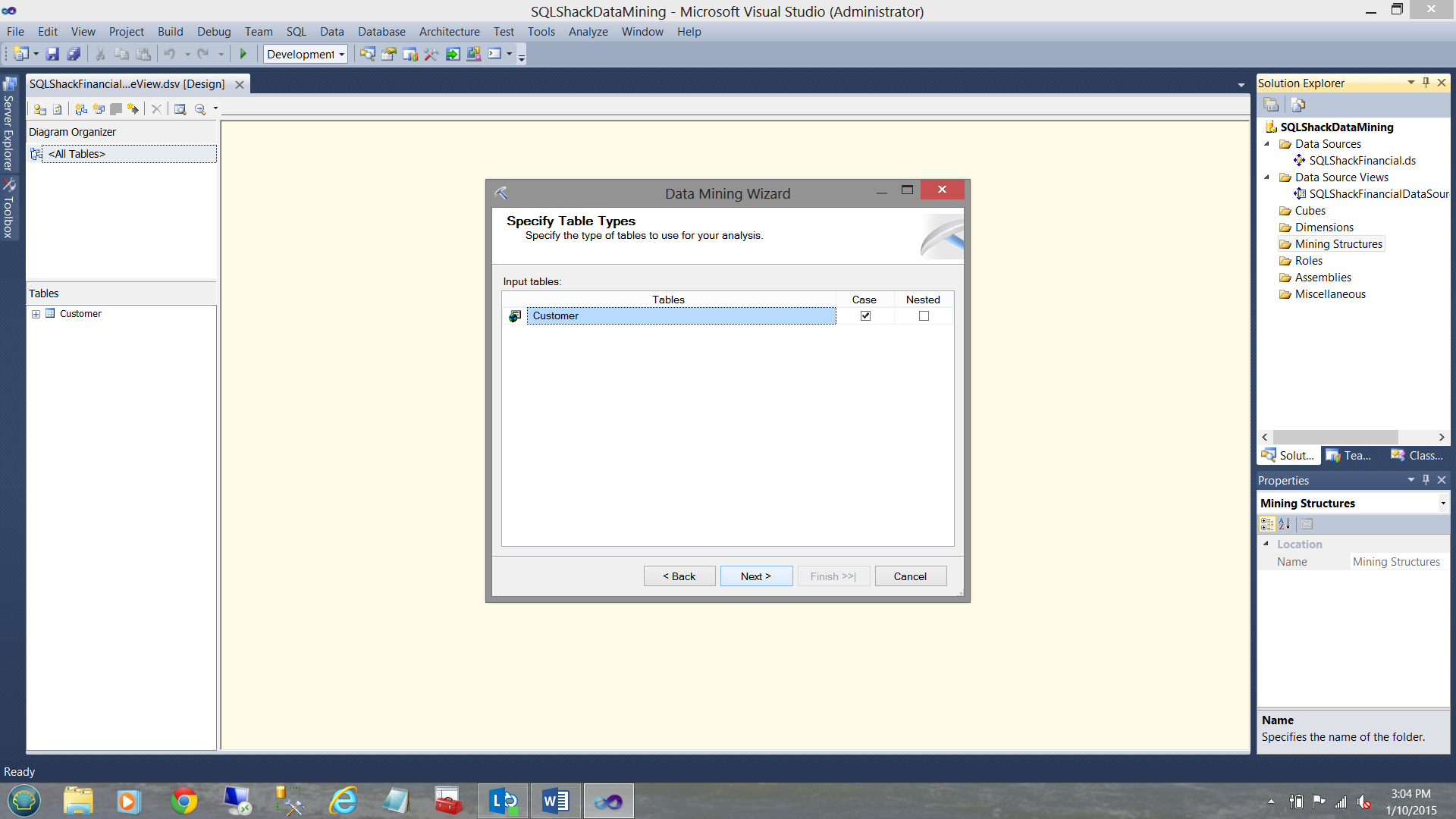
The mining wizard now asks us to let it know where the source data resides. We select the “Customer” table (see above) and we click next.
At this point, we need to understand that once the model is created we shall “process” the model. Processing the model achieves two important things. First it “Trains” the model as to what type of data we are utilizing and runs that data against the data mining model that we have selected. After obtaining the necessary results, the process compares the actual results with the predicted results. The closer the actuals are to the predicted results the more accurate the model that we selected. The reader should note that whilst Microsoft provides us with +/- twelve mining models NOT ALL will provide a satisfactory solution and therefore a different model may need to be used. We shall see just this within a few minutes.
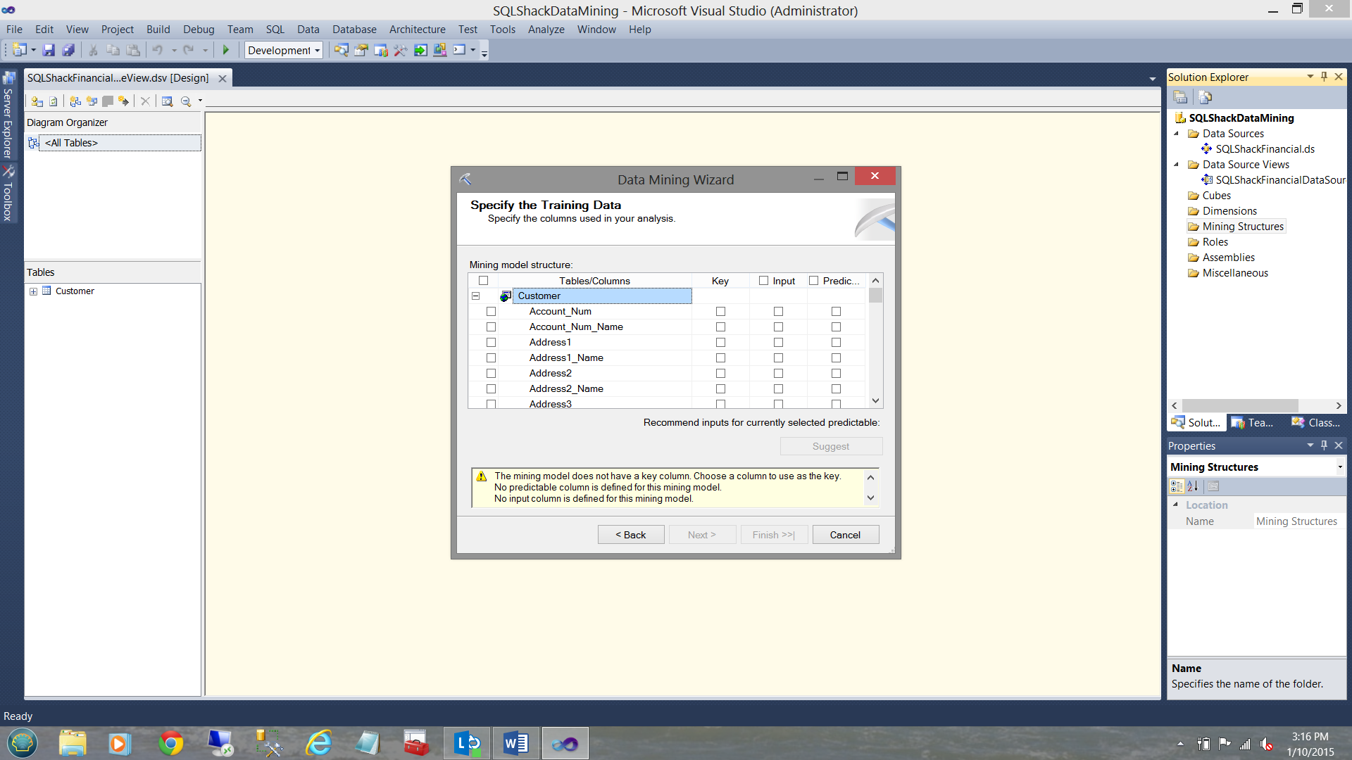
We now must specify the “training data” or in simple terms “introduce the Microsoft mining models to the customer raw data and see what the mining model detects”. In our case, it is the data from the “Customer” table. What we must do is to provide the system with a Primary Key field. Further, we must tell the system what data fields/criteria will be the data inputs that will be utilized with the mining model to see what correlation (if any) there is between these input fields (Does the client owns a house? How many cars does the person own? Is he or she married?) and what we wish to ascertain from the “Predicted” field (Is the person a good credit risk?) .
Setting the Primary Key

For the primary key we select the fields “PK_Customer_Name” (see above).
Selecting the input parameters / fields

We select “Houseowner” and “Marital_Status” (see above)
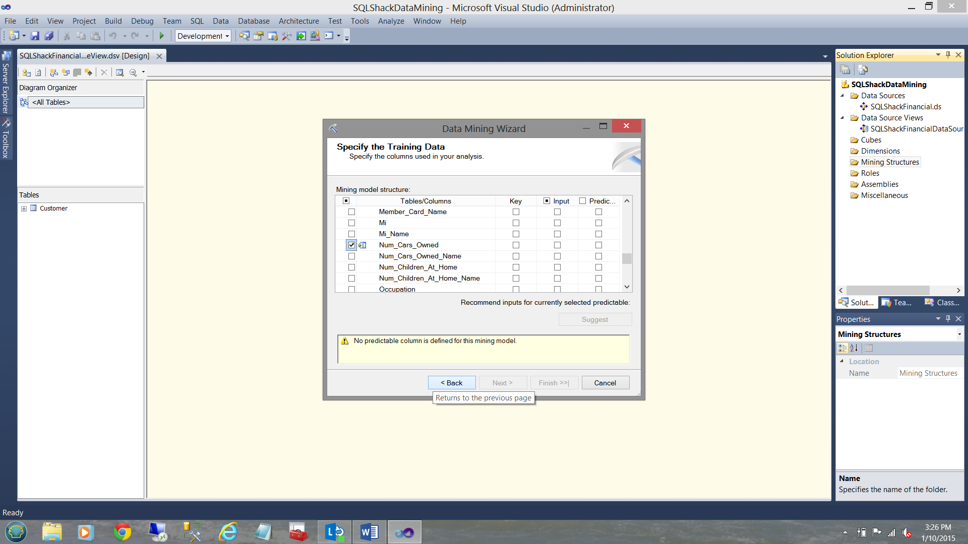
and “number of cars owned” (see above)
As the reader will see from the two screen shots above, we selected
- Does the applicant own a house?
- Is he or she married?
- How many cars does he / she owns.
NOTE that I have not included income and this was deliberate for our example.
Bernie Madoff’s income was large however we KNOW that he would not be a good risk.
Lastly, included within the raw data was a field called Credit Class which are KNOWN credit ratings for the clients concerned.
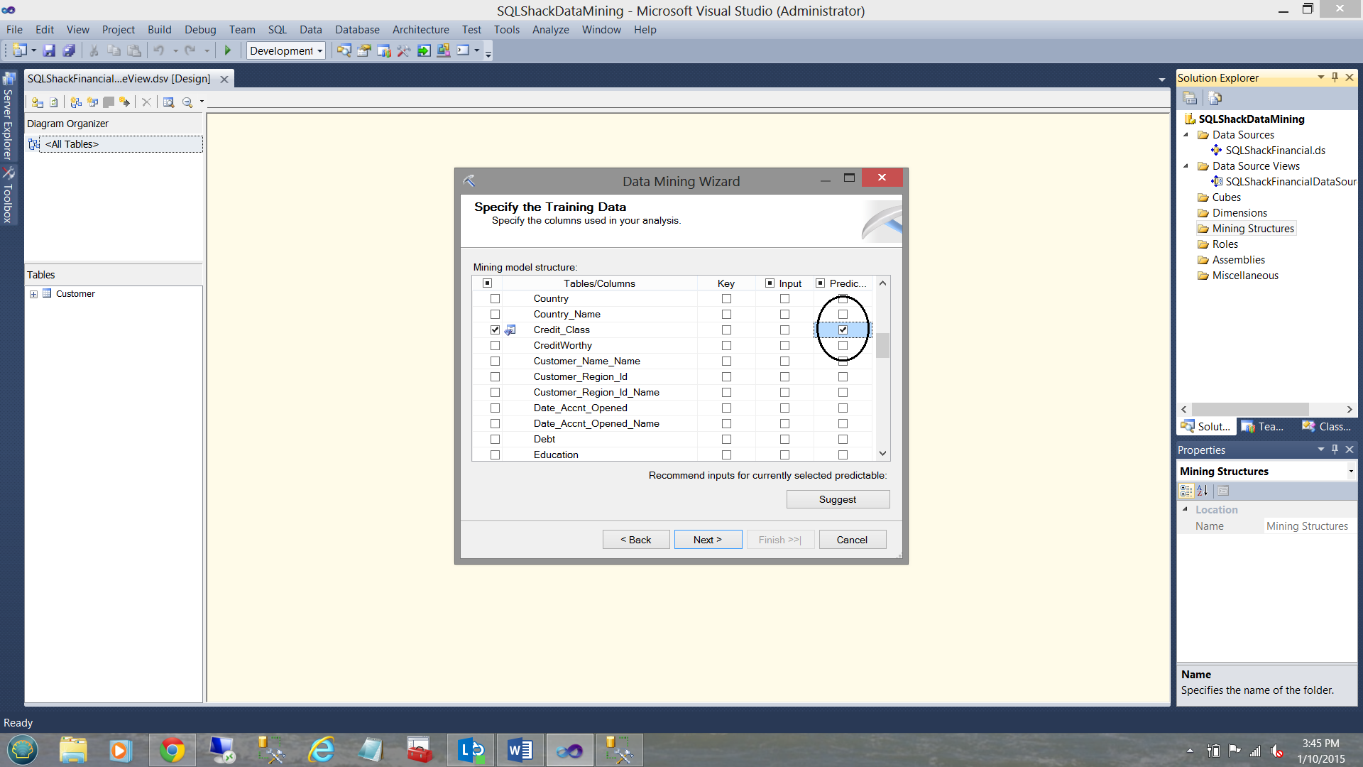
Selecting the PREDICTED field
Last but not least, we must select the field that we wish the mining model to predict. This field is the “Credit Class” as may be seen below:
To recap:
- The primary key is “PK_Customer_name”
- The input parameters are
- Is the person married?
- Is the person a house owner?
- How many cars does the person own?
- The field that we want the SQL Server Data Mining Algorithm to predict is the credit “bucket” that the person should fall into.. 0 being a good candidate and 4 being the worst possible candidate.
We now click “Next”.
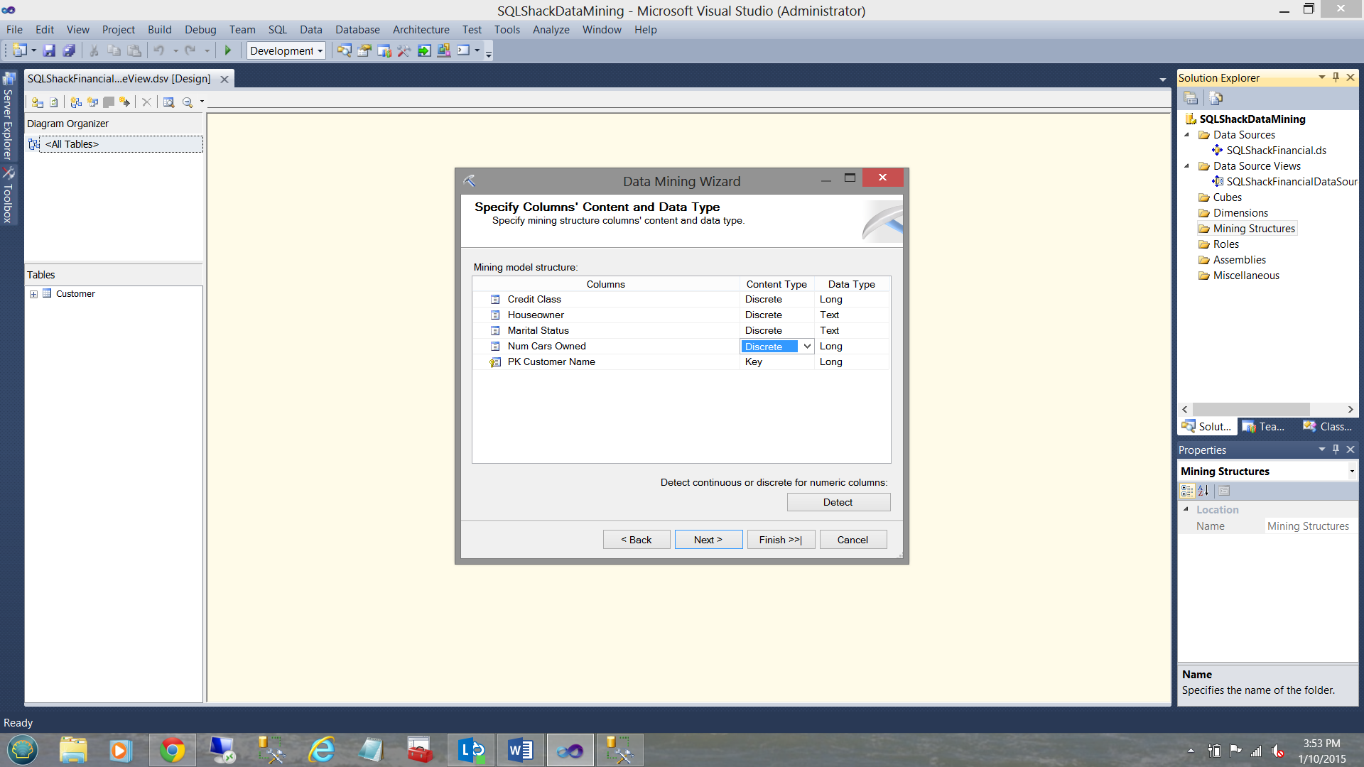
Having clicked “Next we arrive at the “Specify Columns’ Content and Data Type Screen”.
Credit class (the predicted field) is either a 0, 1, 2, 3, 4. These are discrete values (see above).
The number of cars owned is also a discrete value. No person owns 1.2 cars.
House Owner is a Boolean (Y or N).
Marital (Married) status is also a Boolean Value (Y or N).
We click next.
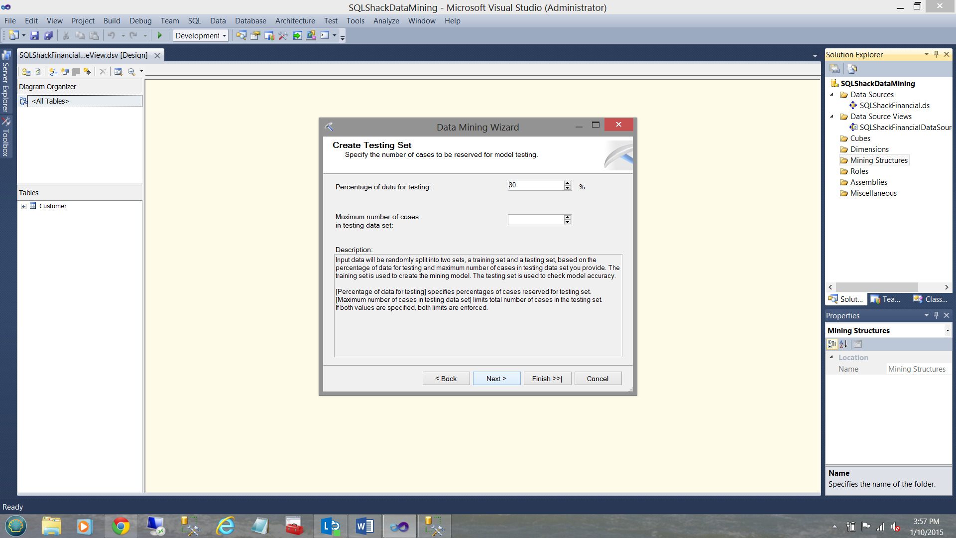
SQL Server now wishes to know of all the records within the customer table, what percentage of the data (RANDOMLY SELECTED BY THE MINING ALGORITHM) should be utilized to test just how closely the predicted values of “Credit class” tie with the actual values of “Credit Class”. One normally accept 30% as a good sample (of the population). As a reminder to the reader, the accounts within the data ALL have account numbers under 25000. We shall see why I have mentioned this again (in a few minutes).
We then click next.
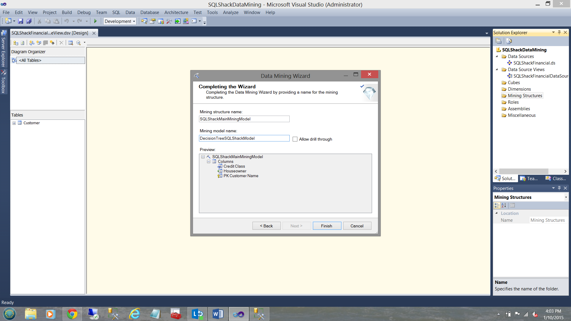
The system wants us to give our mining model a name. In this case, we choose. “SQLShackMainMiningModel”. This is the “mommy”. “SQLShackMainMiningModel” has four children, one being the Decision Tree algorithm that we just created and three more which we shall create in a few moments. For the mining model name, we select “DecisionTreeSQLShackModel”.
We now click “Finish”.
We are returned to our main working surface as may be seen above.
Creating the remaining three models
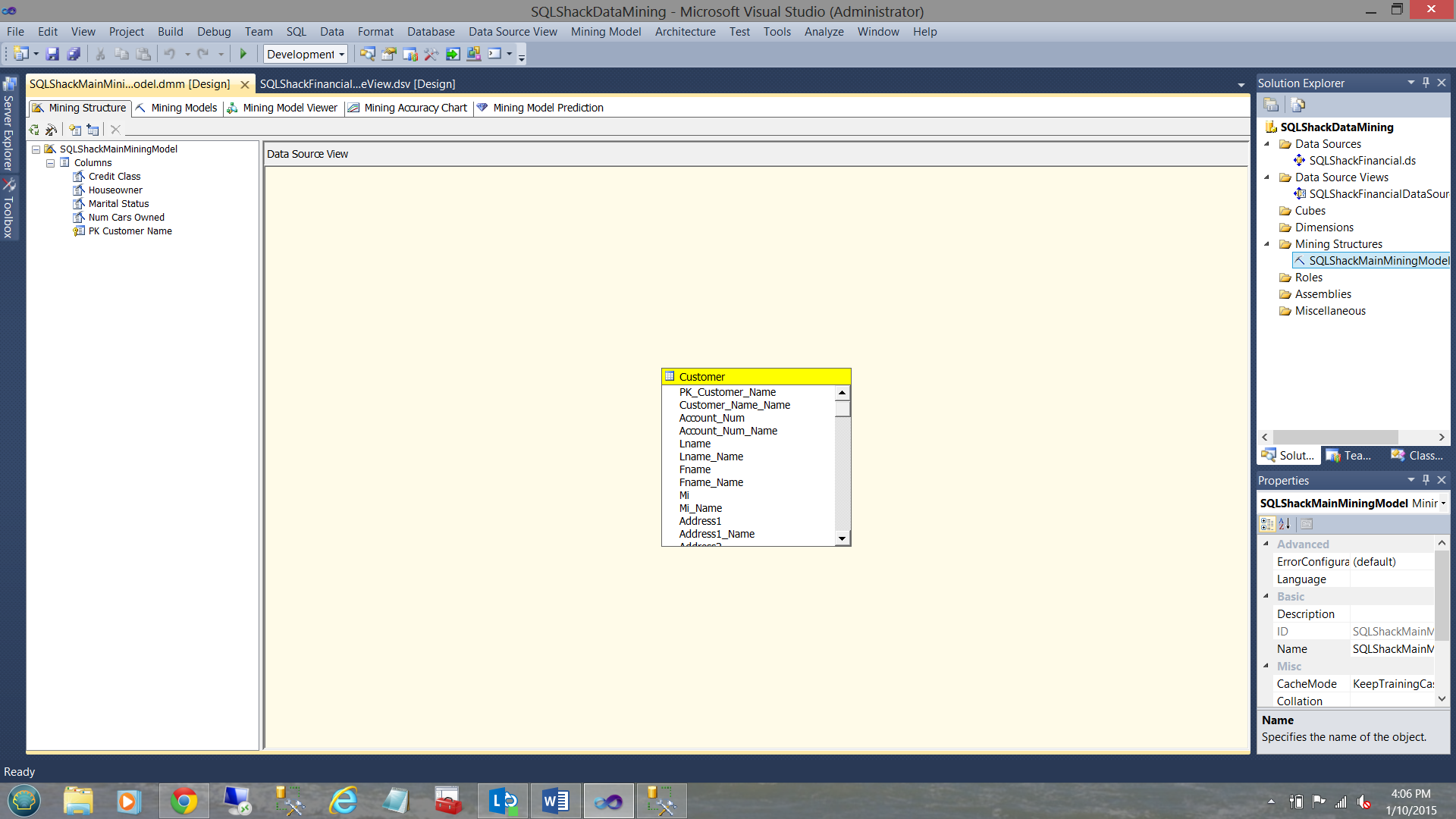
From the “Mining Structures” folder we double-click our “SQLShackMainMiningModel” that we just created.
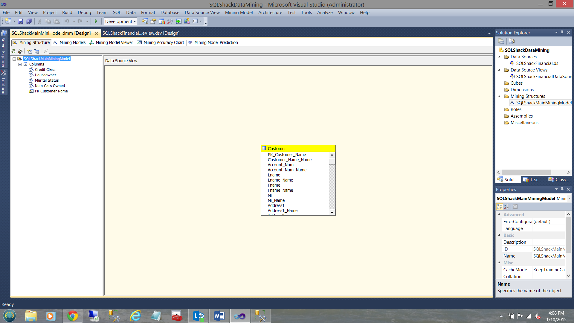
The “Mining Structure” opens. In the upper left-hand side, we can see the fields for which we opted. They are shown under the Mining structure directory (see above).
Clicking on the “Mining Models” tab, we can see the first model that we just created.
What we now wish to do is to create the remaining three models that we discussed above.
The first of the three will be a Naïve-Bayes Model. This is commonly used in a predictive analysis. The principles behind the Naïve-Bayes model are beyond the scope of this paper and the reader is redirected to any good predictive analysis book.
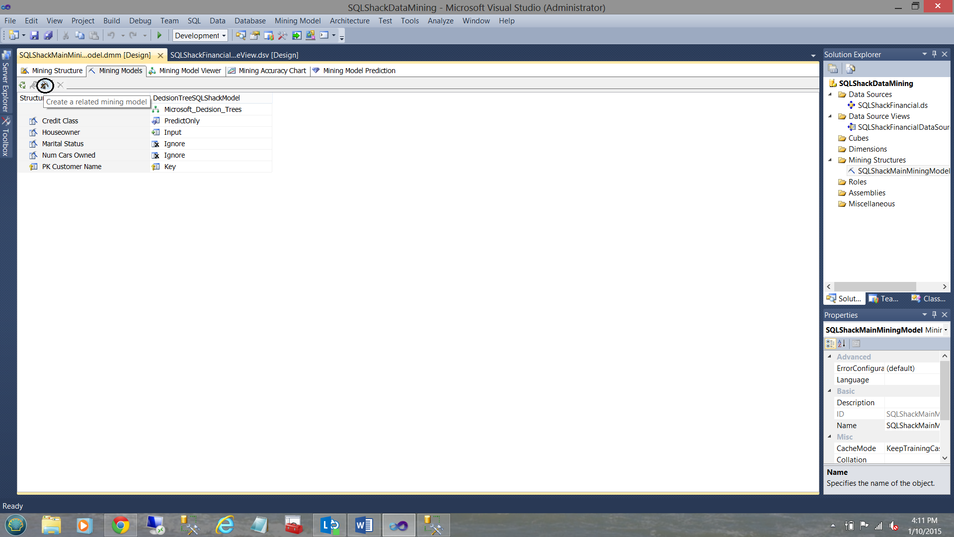
We select the “Create a related mining model” option (see above with the pick and shovel).
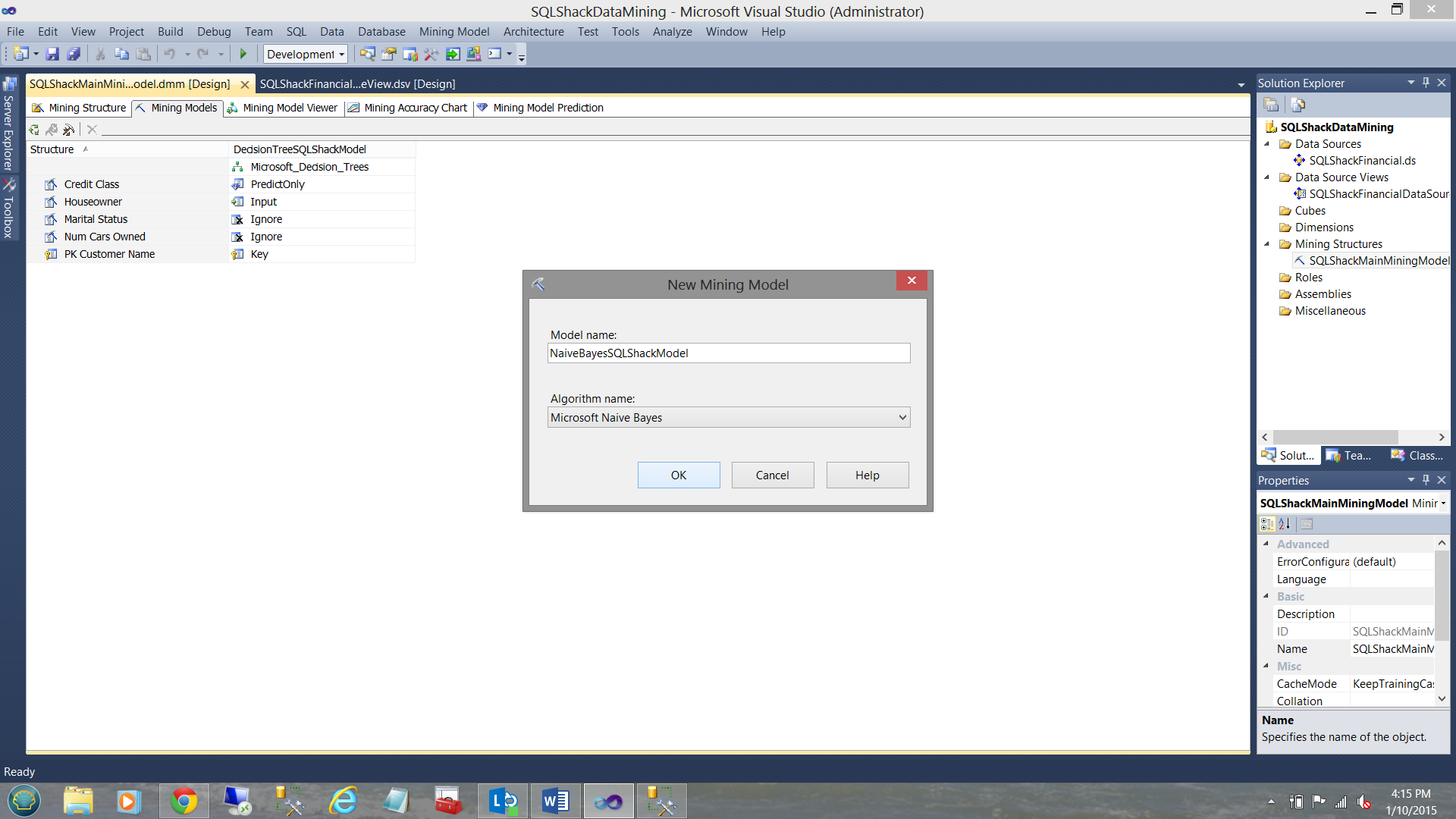
The “New Mining Model” dialogue box is brought up to be completed (see above).
We give our model a name and select the algorithm type (see above).
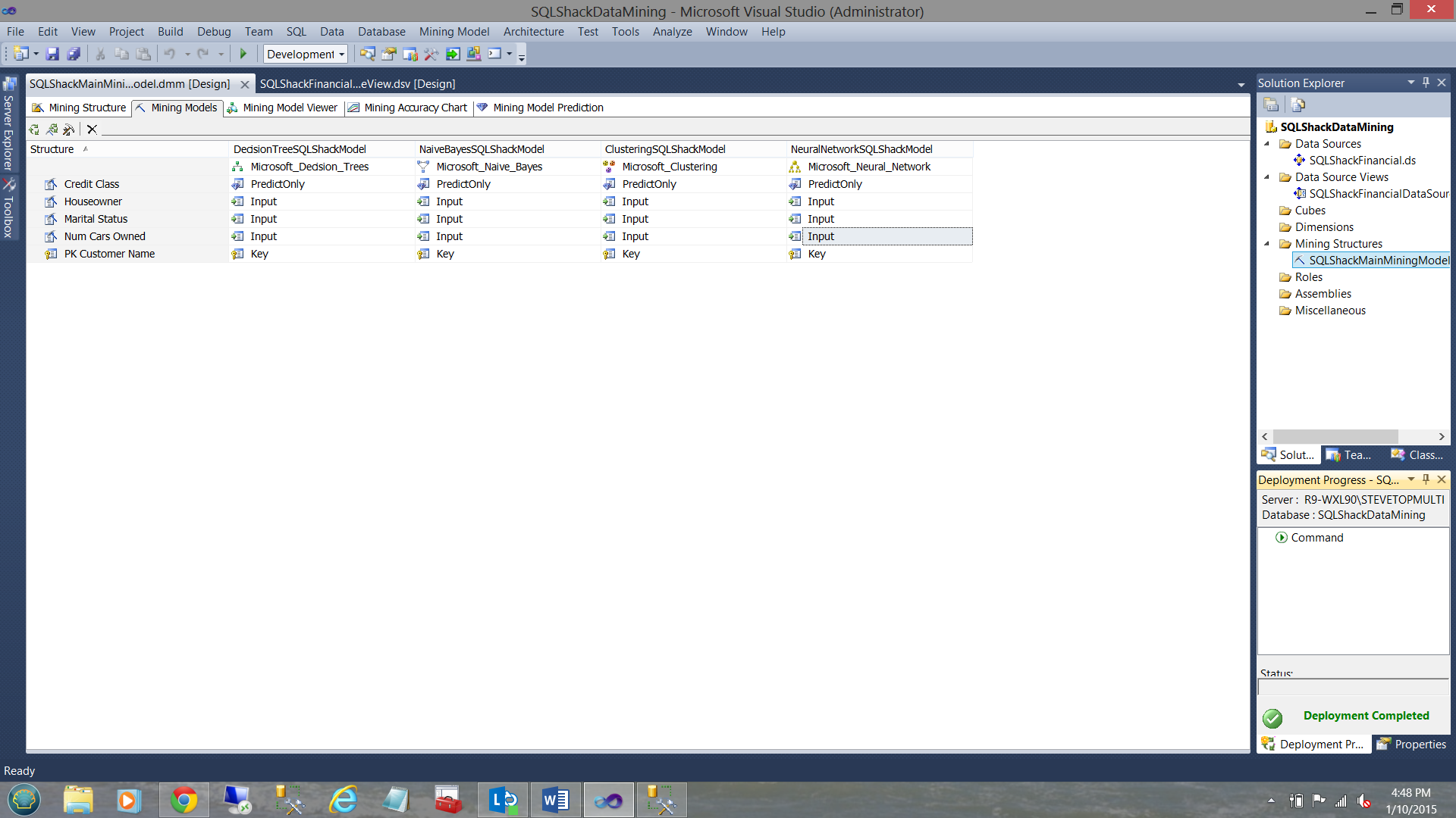
In a similar manner, we shall create a “Clustering Model” and a “Neural Network”. The final results may be seen below:
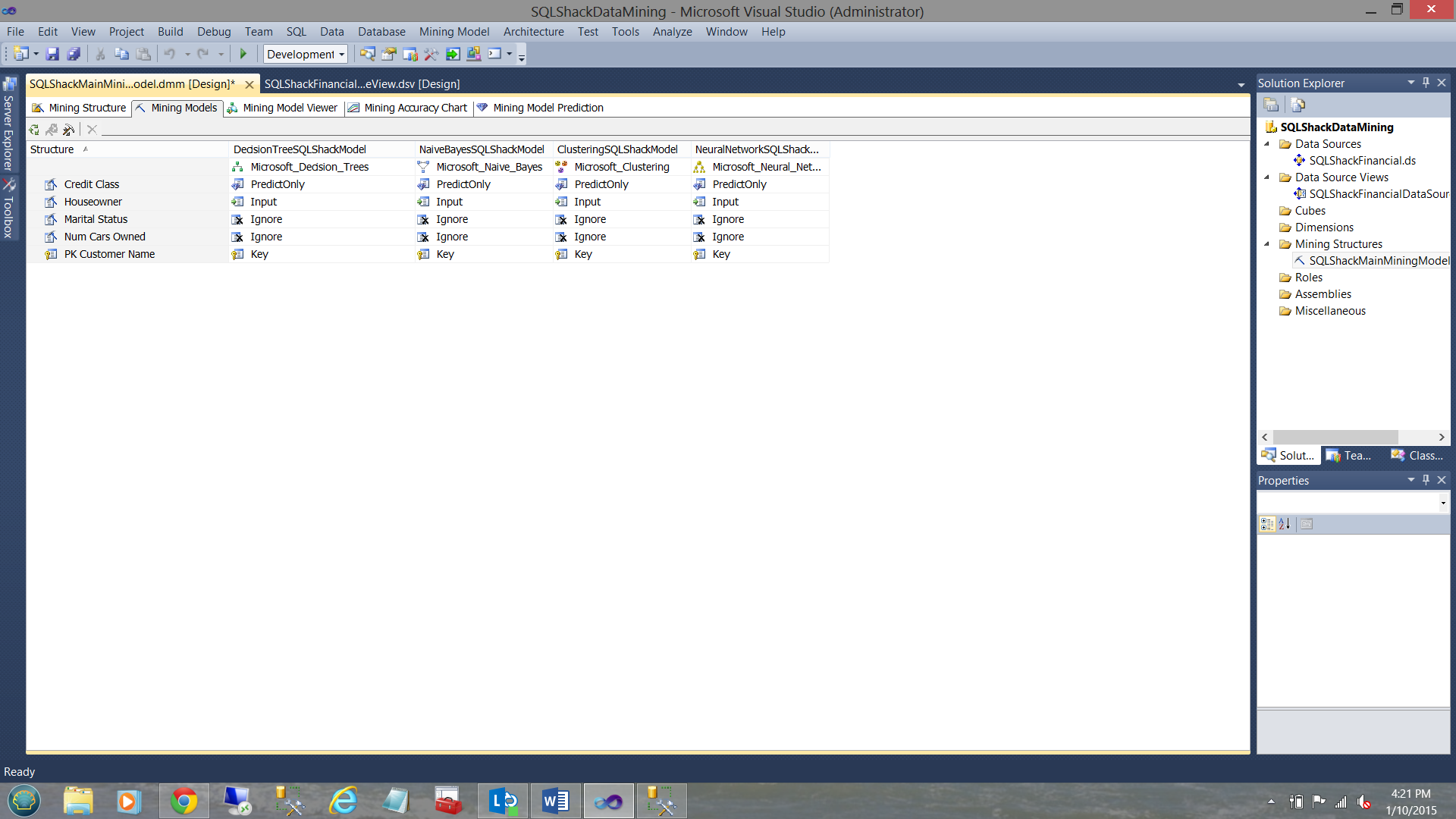
We have now completed all the heavy work and are in a position to process our models.
Setting the properties of the Analysis Services database
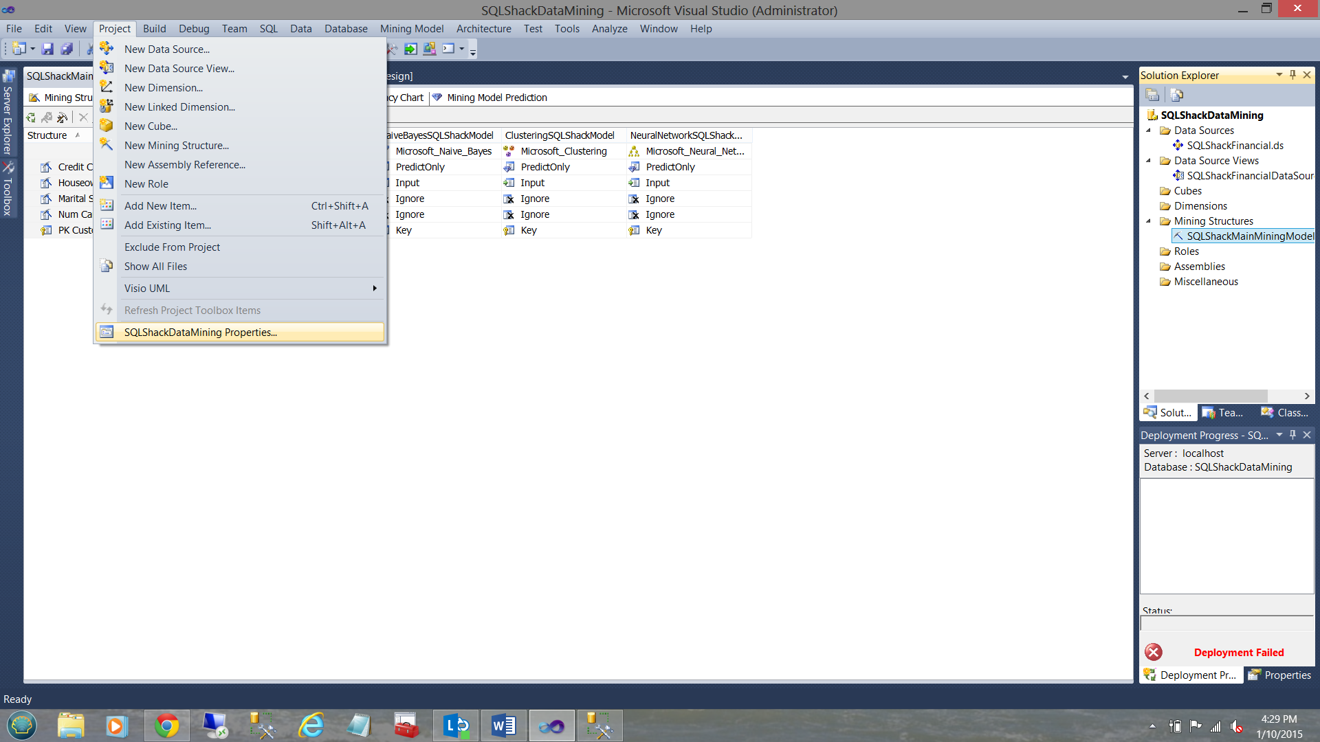
We click on the “Project” tab on the main ribbon and select “SQLShackDataMining” properties (see above).
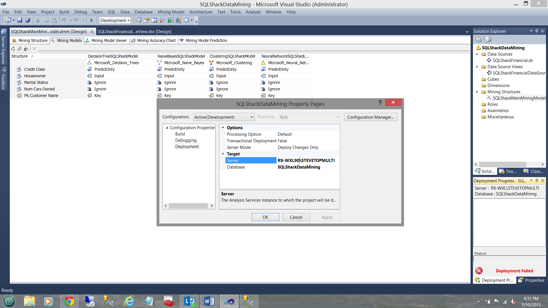
The “SQLShackDataMining Property Pages” are brought into view. Clicking on the “Deployment” tab, we select the server to which we wish to deploy our OLAP database, and in addition, give the database a name.
We then click “OK”.
Processing our models
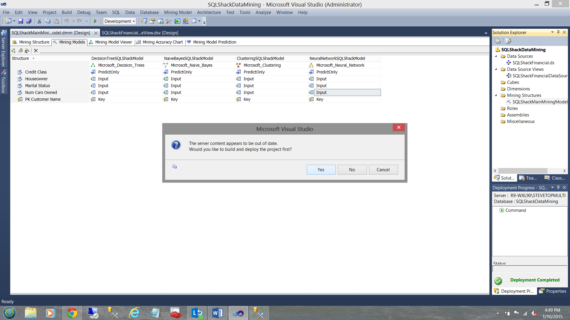
We right click on the “SQLShackMainMiningModel” and select “Process”.
We are told that our data is old and do we want to reprocess the models (see below).

We answer “Yes”.
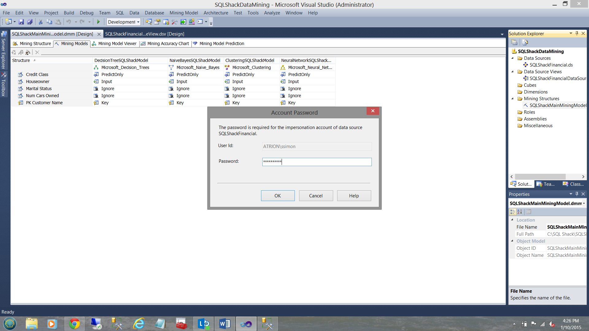
We are then asked for our credentials (see above). Once completed, we select “OK”.
One the build is complete, we are taken to the “Process Mining Structure” screen. We select the run option found at the bottom of the screen (see below in the blue oval).
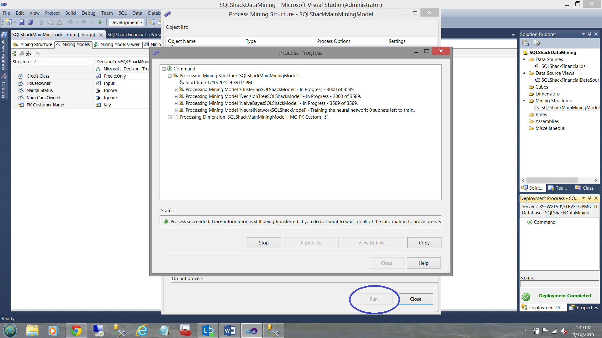
Processing occurs and the results are shown above.
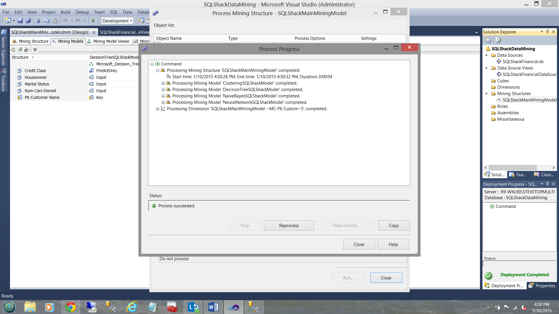
Upon completion of processing, we click the “Close” button to leave the processing routine (see above). We now find ourselves back on our work surface.
Let the fun begin!!
Now that our models have been processed and tested (this occurred during the processing that we just performed), it is time to have a look at the results.
We click on the third tab “Mining Model Viewer”
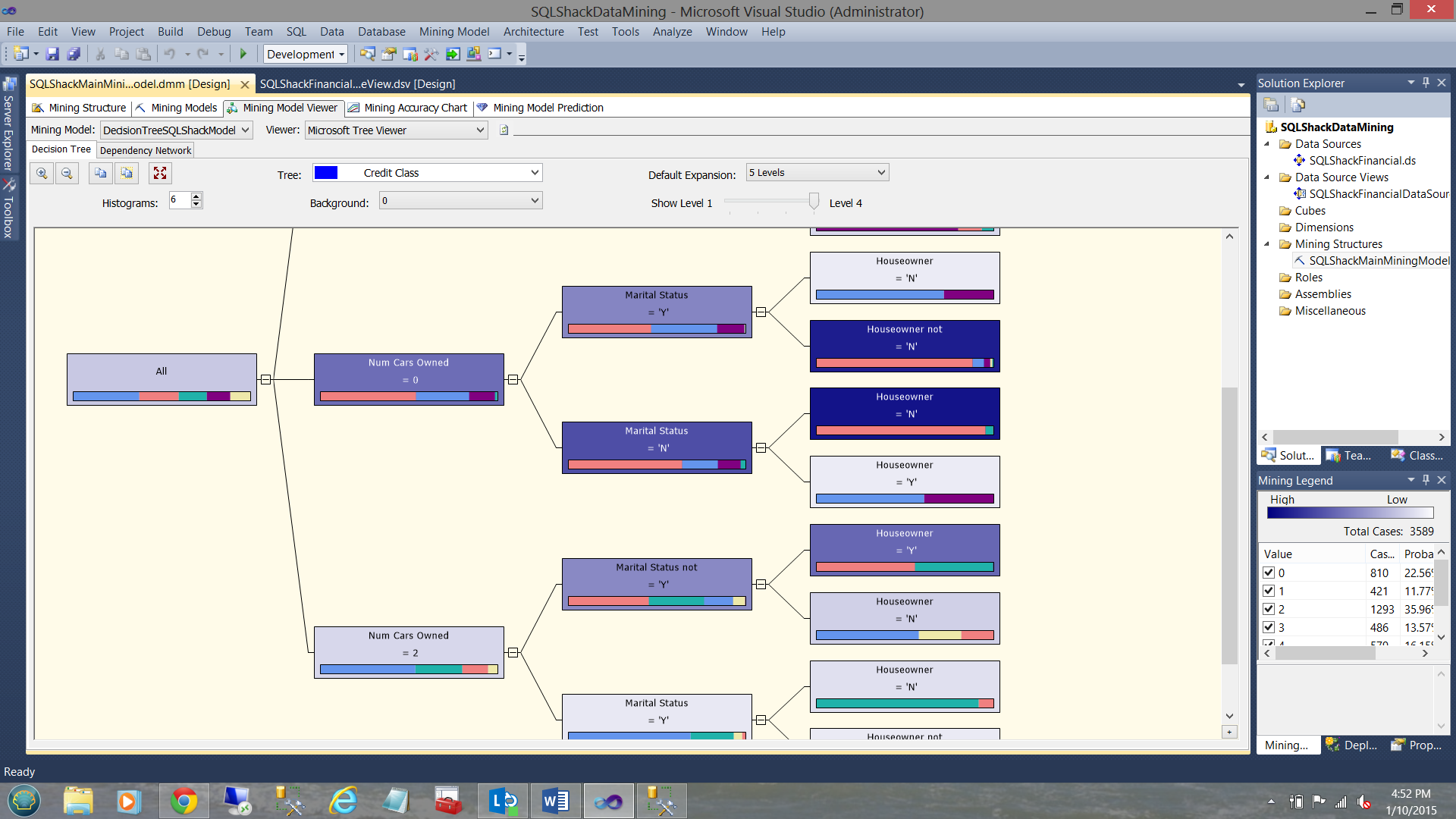
Selecting our “Decision Tree” model as a starting point, we select zero as our background value. The astute reader will remember that zero is the best risk from our lending department. THE DARKER THE COLOUR OF THE BOXES is the direction that we should be following (according to the predicted results of the processing).
That said, we should be looking at folks who own no cars, are not married and do not own a house. You say weird!! Not entirely. It can indicate that the person has no debt. We all know what happens after getting married and having children to raise 🙂
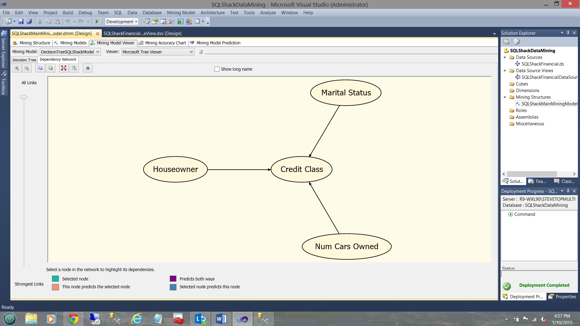
Clicking the “Dependency Network” tab we see that the mining model has found that the credit class is dependent Houseowner, Marital Status and Num Cars Owned.
By sliding the “more selective” slider found under the text “All Links” (see above) we are telling the model to go down to the grain of the wood “to see which one of the three is the most decisive” in determining the relationship between it and the credit class (see below).
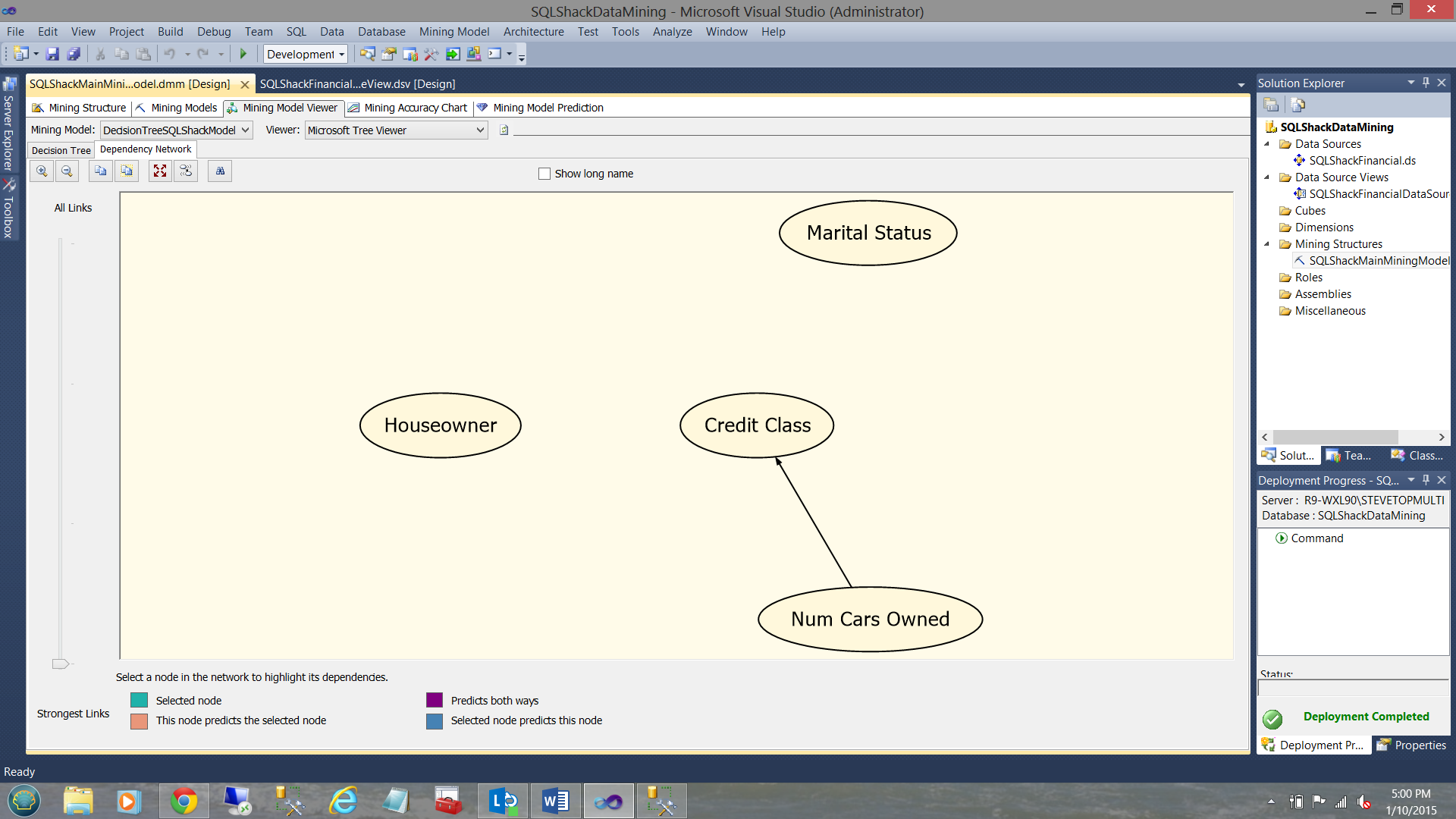
We note that “Num Cars Owned” seems to play a major role. In other words, the mining model believes that there is a strong relationship between the credit class and the number of cars that the person either owns OR is currently financing. Now the “doubting Thomas” will say why? Mainly because cars cost money. Most people finance the purchase of cars. Credit plays a big role in financing.
The remaining three algorithms
A full discussion of all four algorithms, how they work and what to look for to justify selecting any of the four (over and above the others) is certainly in order, however in the interests of brevity and driving home the importance of data mining itself, we shall put this discussion off until a future get together.
We shall, however, continue to see how the system has ranked these algorithms and which of the four the process recommends.
The Mining Accuracy Chart
Having now created our four mining models, we now wish to ascertain which of the four have the best fit for our data and has the highest probability of rendering the best possible information.
We click on the “Mining Accuracy Chart” tab
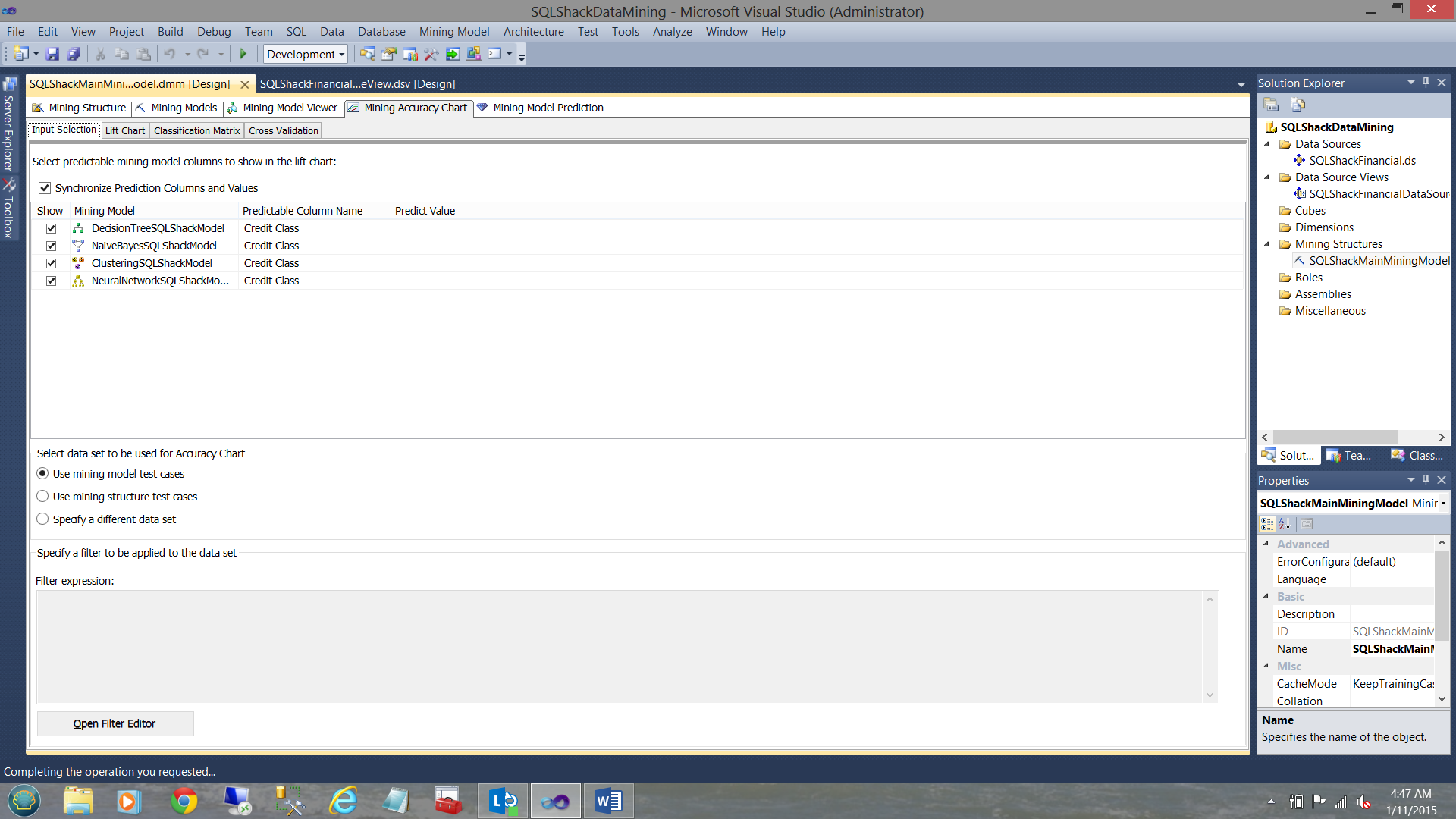
Note that the accuracy chart has four tabs itself. The first of the tabs is the “Input Selection”. We also note that our four mining models are present on the screen (see above).
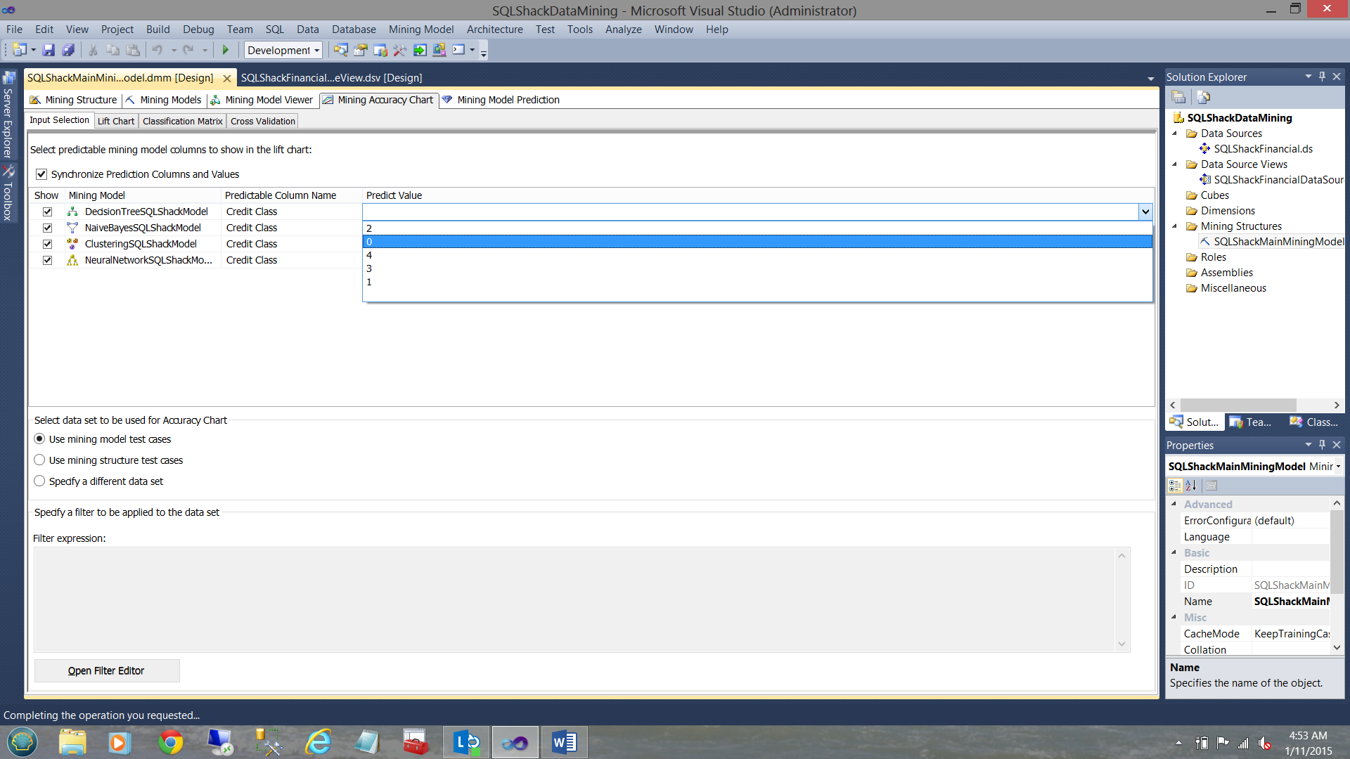
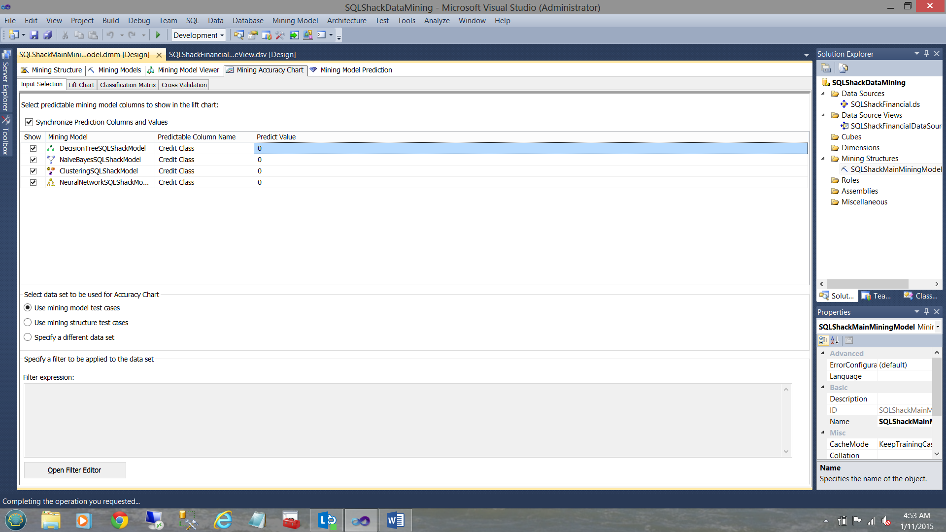
As SQLShack financial makes most of its earnings from lending money and as we all realize that they wish to lend funds to only clients that they believe are a good risk (i.e. a rating of 0 ), they set the “Predict Value” to zero for all four algorithms (see below).
and when complete, our screen should look as follows (see below):
The astute reader will note that in the lower portion of the screen we are asked which dataset we wish to utilize. We accept the dataset “the mining model test cases” used by the system in the creation of our model. Later in this discussion, we shall utilize data that we have held back from the model to verify that the mining models hold for that data as well. That will be the proof of the pudding!
The Lift Chart
The lift chart (in my humble opinion) tells all. Its purpose is the show us which of the four models the system believes is the best fit for the data that we have.
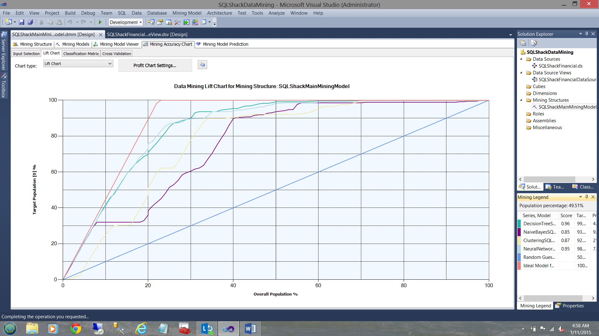
I like to call the Lift Chart “the race to the top”. It informs us how much of the population should be sampled (check their real credit rating) to make a decision on the credit risk which is most beneficial to SQLShack Financial. In simple terms, it is saying to us “This model requires checking x% of the population before you can be fairly certain that your model is accurate”. Keeping things extremely simple, the lower the required sampling amount, the more certain that one can be that the model is accurate and is, in fact, one of the models that we should be utilizing.
That said, the line graph in pink (see above) is a line generated by the mining structure processing. It shows the best possible outcome. It essentially is telling us “with the best possible LUCK, we only need to check the true credit ratings of 22% of our applicants”. The light blue undulating lines represent the “Decision Tree” model and the “Neural Network” model and they peak (reach one hundred percent on the Y axis at a population sampling of just over 50 % (X-axis see the graph above). This said they are the most promising algorithms to use. The “Naïve Bayes” and “Clustering algorithms” peak closer to 100% on the X-axis and are therefore not as reliable as the “Decision Tree” and the “Neural Network” algorithms. The straight line in blue from (0,0) to (100,100) is the “Shear dumb luck” line. Enough said. More on accuracy in a few minute. Please stay tuned.
The Classification Matrix
As proof of our assertions immediately above, we now have a quick look at the next tab, the “Classification Matrix”
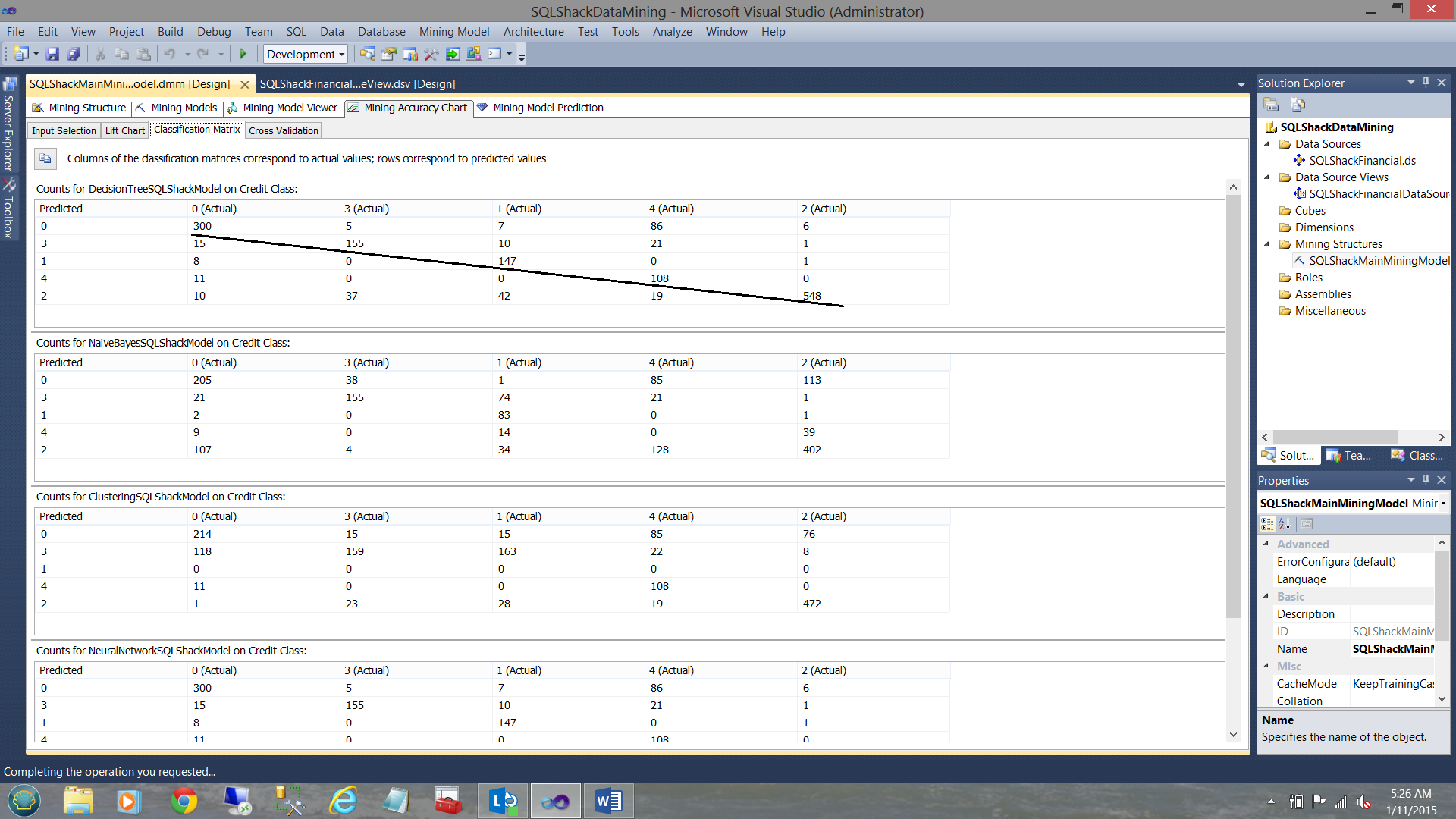
In this fantastic and informative tool, the model shows us how many instances the system found “where the ‘predicted’ was the SAME as the ‘actual’”. Note the first matrix for the “Decision Tree” (the first matrix) and note the strong diagonal between the “Actuals” on the X axis and the “Predicted” on the Y-axis. The same is reasonably true for the “Neural Network” model (see the bottom of the screenshot below).
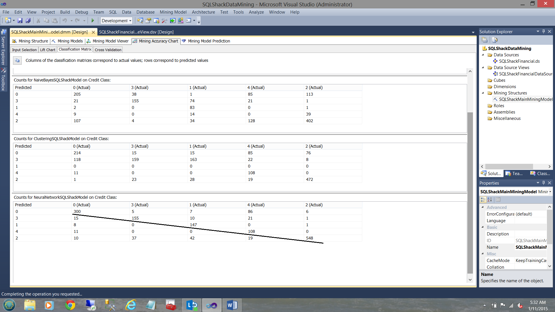
The reader will note that the predicted vs. actuals for the remaining two models are randomly dispersed. The more the entropy, the more doubtful the accuracy of the model (with regards to our data).
Utilizing the Mining Models and verifying their results
At this point, we supposedly have two relatively reliable models with which to work. What we now must do is to verify the predicted versus the actuals. As a reminder to the reader, the only way to ensure that our algorithms are yielding correct predictions is by comparing what “they say” with the “truth” from other credit agencies. The more that match, the more accurate the algorithm will be in predicting; as more and more data is added to our systems.
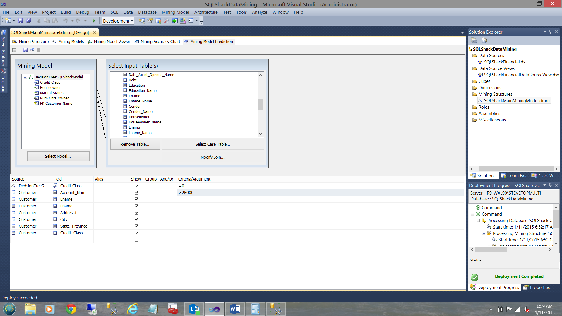
We now click on the “Mining Model Predictions” tab.
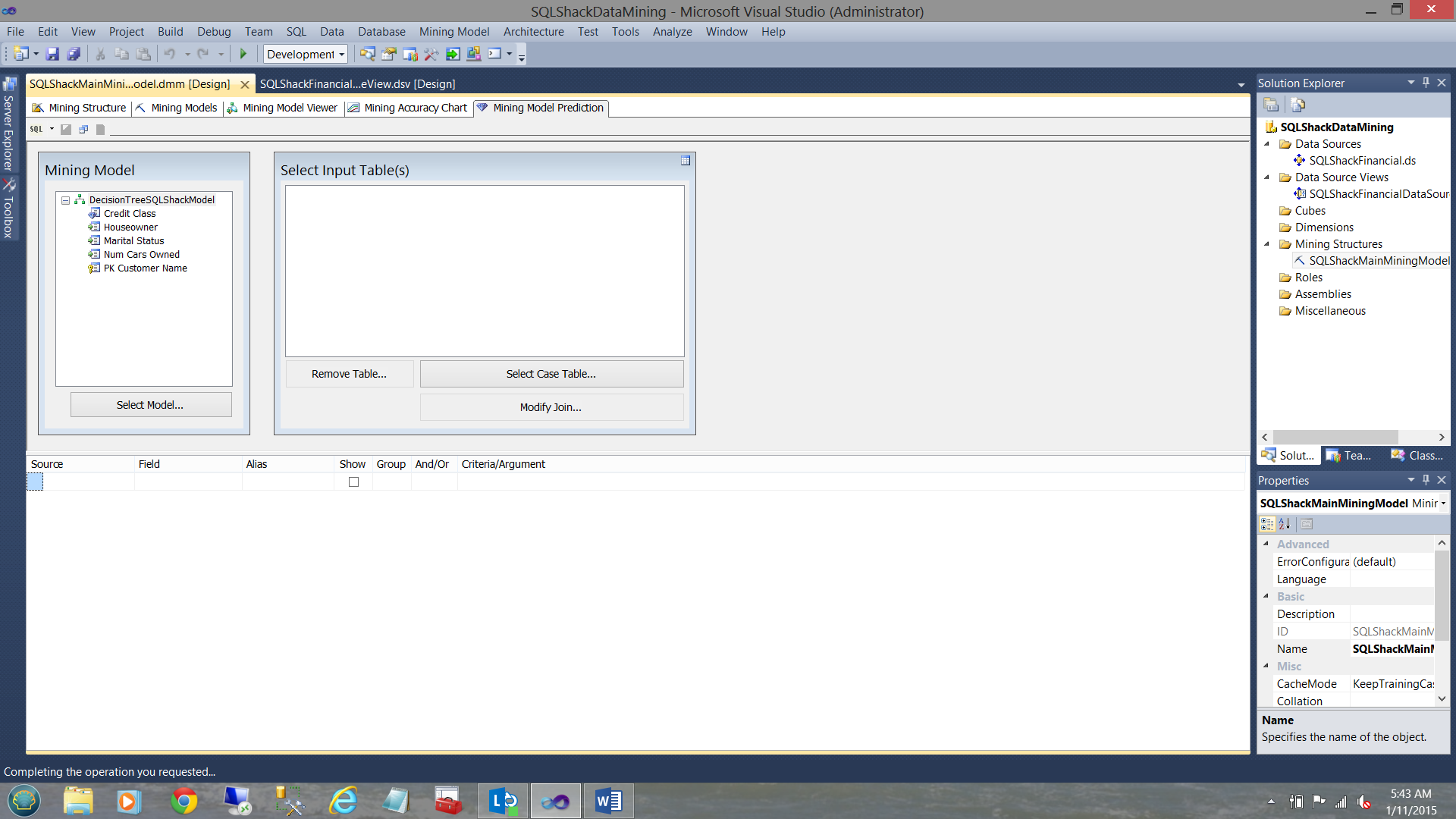
We note that “Decision Tree” model has been selected. Obviously, we could have selected one of the other models but in the interest of brevity, we choose to look at the “Decision Tree”. We must now select the physical input table (with all its records) that we wish the model to act upon.
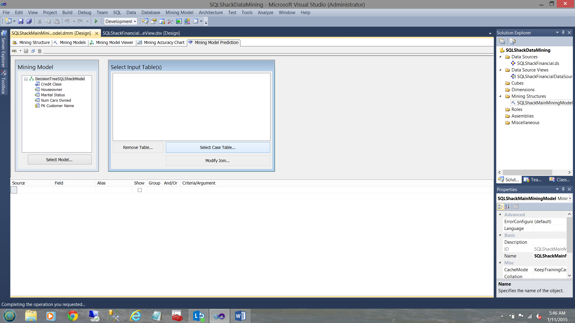
We click “Select Case Table” as shown above and select the “Customer” table (see below).

Note that the fields of the mining model are joined to the actual field of the “Customer” table. What is now required, is to remove the link from the credit class of the model to the actual credit class in the relational table. The field in the table being the known credit class. Simplistically we want the model to predict the credit class, and we shall then see how many matches we obtain.
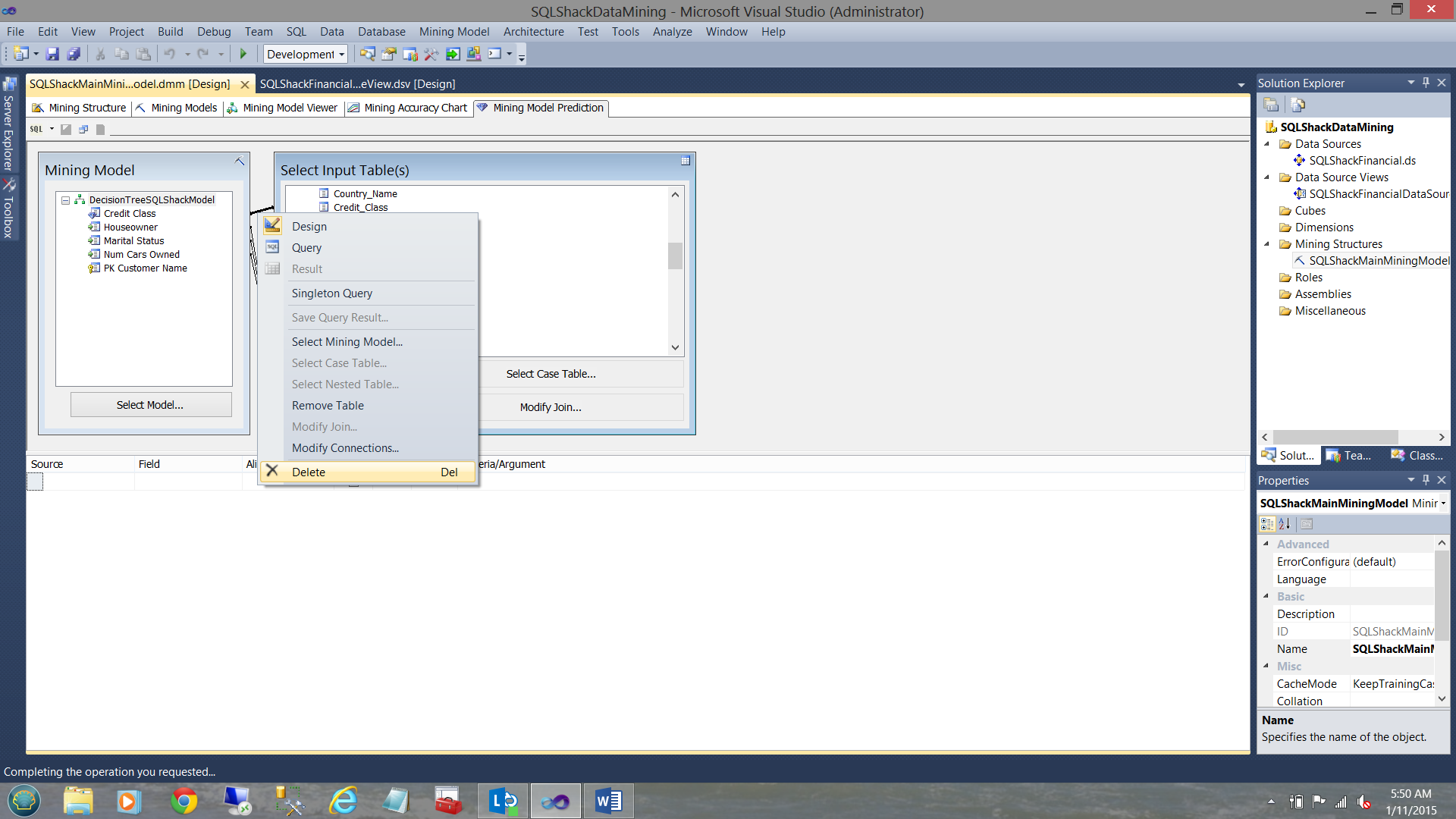
We right click on the credit class link and delete it (see above).
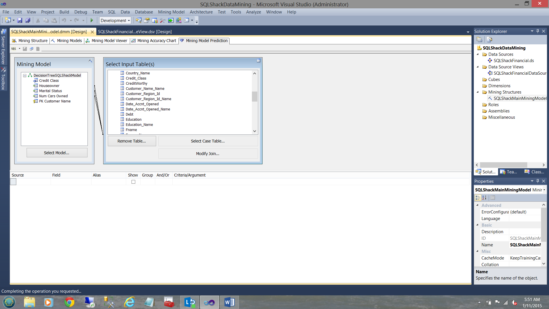
Our screen now looks as follows (see above).
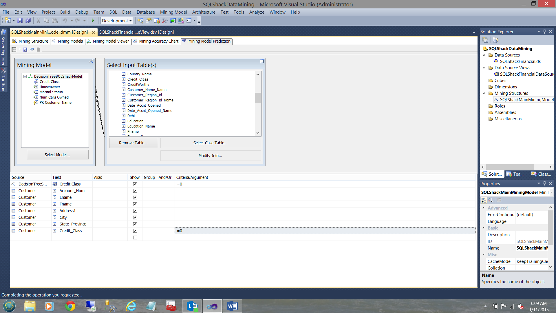
We are now in a position to create our first Data Mining Query (DMX or Data Mining Expression) to “prove out” our model.

In the screen above we select the first field to be the “Credit Risk” from the data mining model.
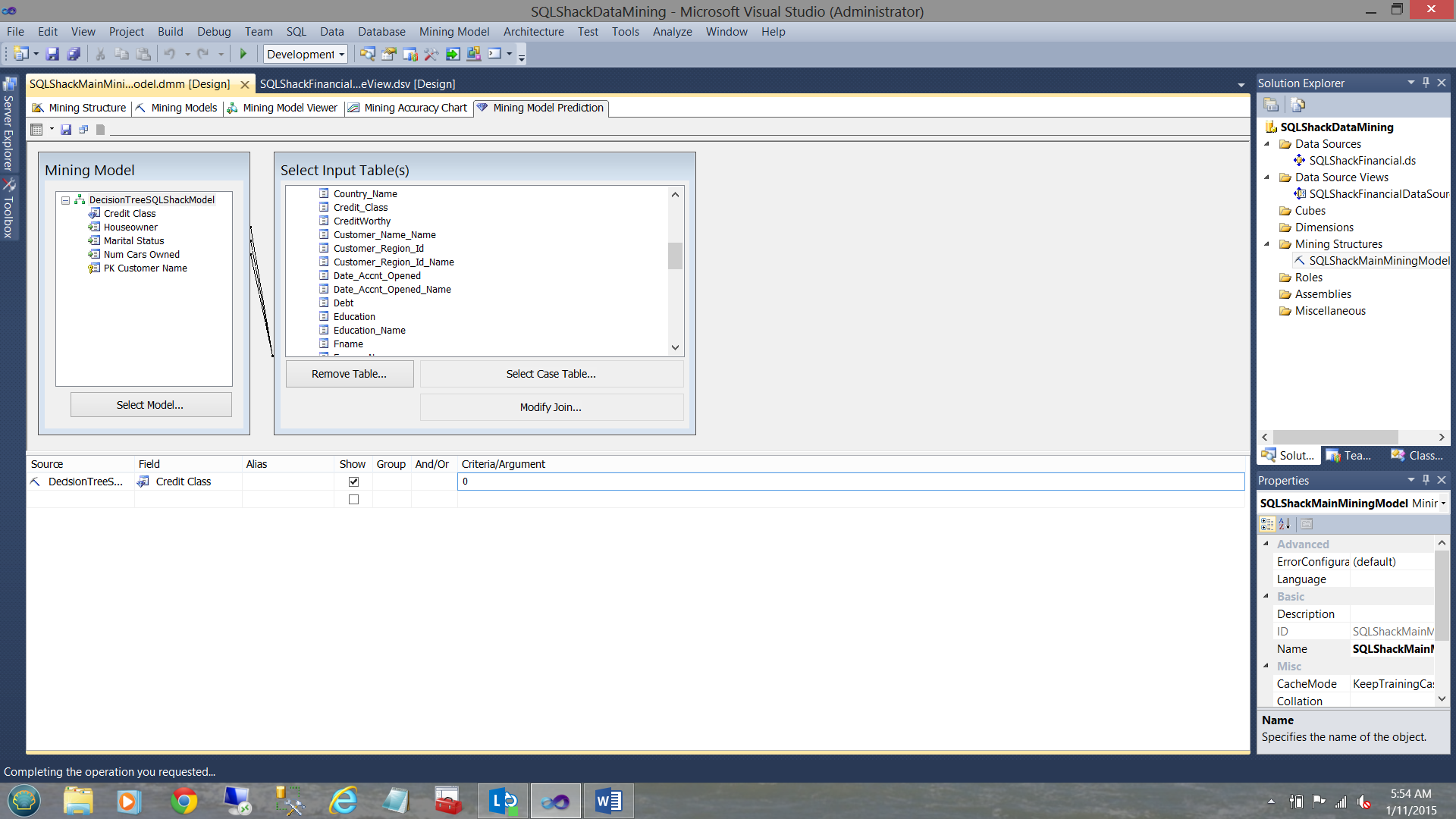
We set its “Criteria / Argument” to 0 (see above).
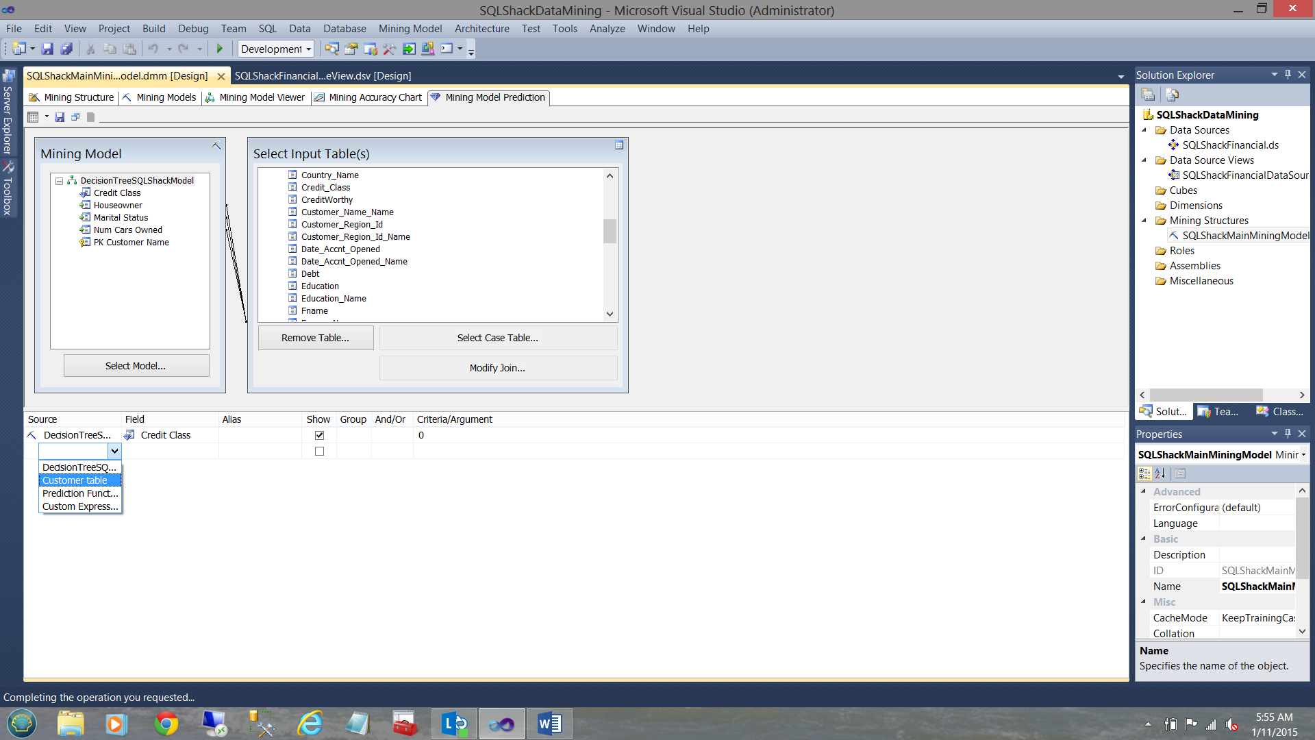
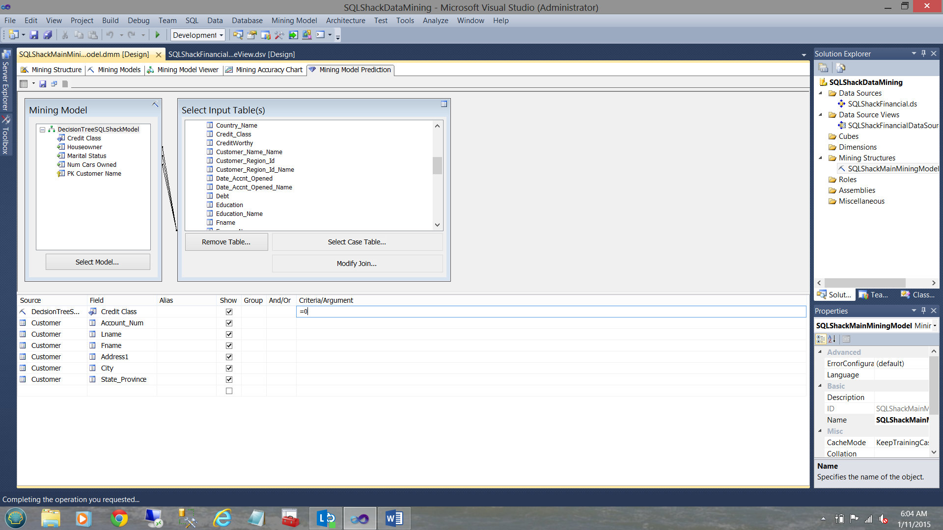
We now add more fields from the “Customer” table to identify these folks!

We have now added a few more fields (from the source table) as may be seen above. Let us see what we have.
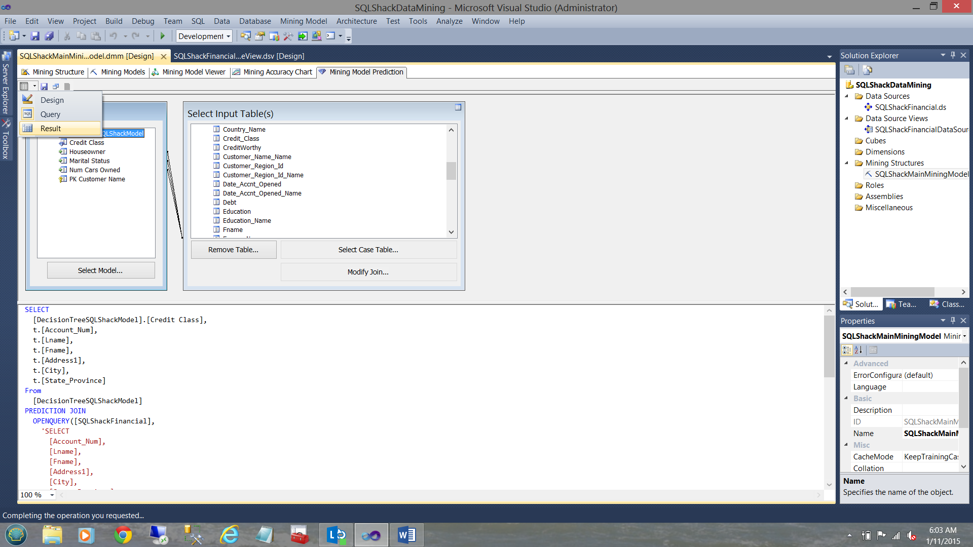
Under the words “Mining Structure” (upper left in the screen shot above) we click on the drop down box. We select the “Query” option (see below).
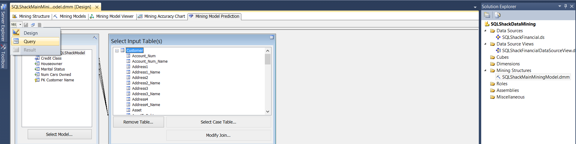
The resulting DMX code from our design screen is brought into view.
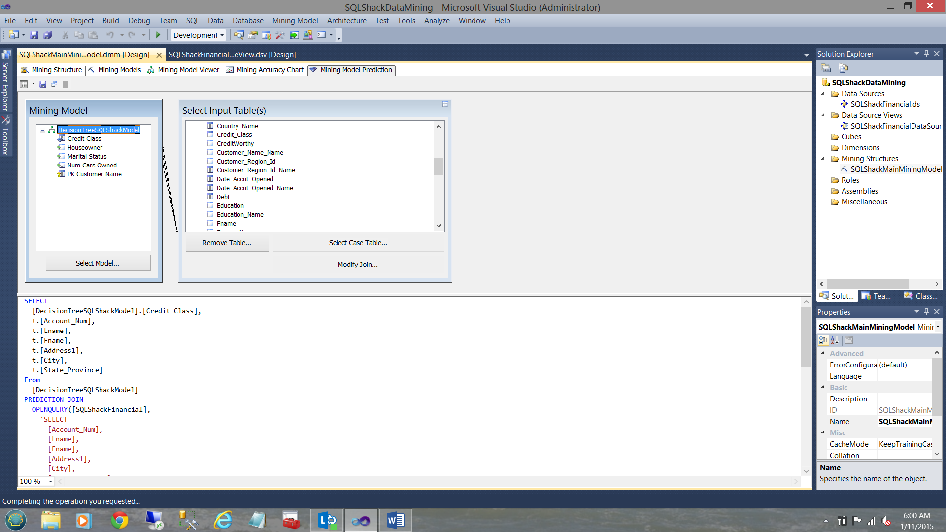
This DMX code should not to be confused with MDX code. Personally I LOVE the feature of having access to the code, as now that we have the code, we can utilize this code for reporting. More about this in my next part of this article.
Once again we select the drop down box below the words “Mining Structure” and select “Result” (see below).
We now obtain our result set.
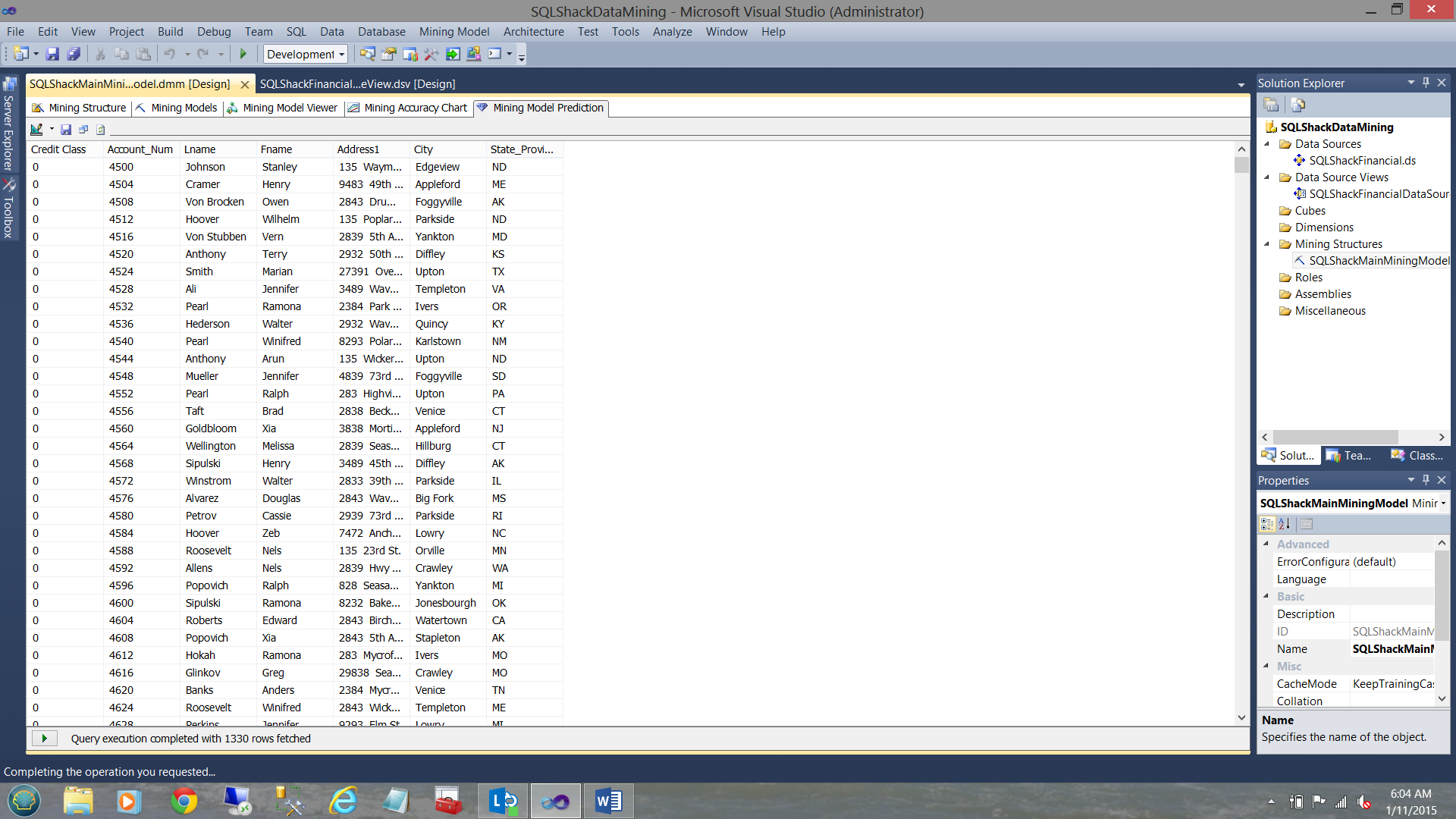
We note that the model has rendered 1330 rows that it believes would be a good credit risk.

Let us now throw a spanner into the works and add one more field to the mix. This field is the TRUE CREDIT RISK and we shall tell the system that we wish to see only those records whose “true credit risk” was a 0. In short, actual equals predicted.
Our design now looks as follows.
Running our query again, we now find that:

994 rows were returned, that the algorithm predicted would be a 0 and were, in fact, a credit class of 0. This represents 74.7% accuracy which is surprisingly good.
Fine and Dandy!!
Thus far we have performed our exercises with account numbers less than 25000.
Let us now add a few more accounts. These accounts will have account numbers over 25000. We now load these accounts and reprocess the results. We now set up our query as follows (see below).
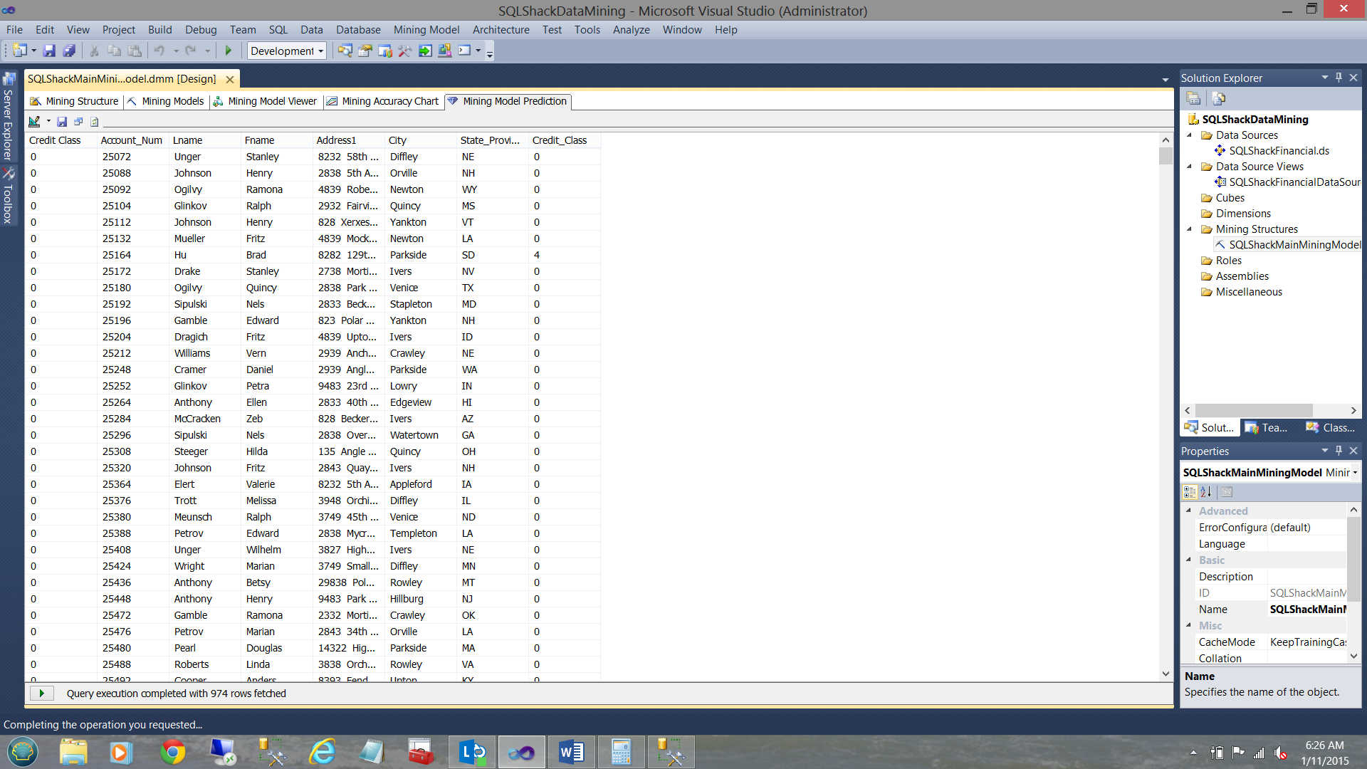
The result set may be seen above. We retrieved 974 rows.

Changing this query slightly and once again telling the query to only show the rows where the predicted and actual credit classes are 0 we find…
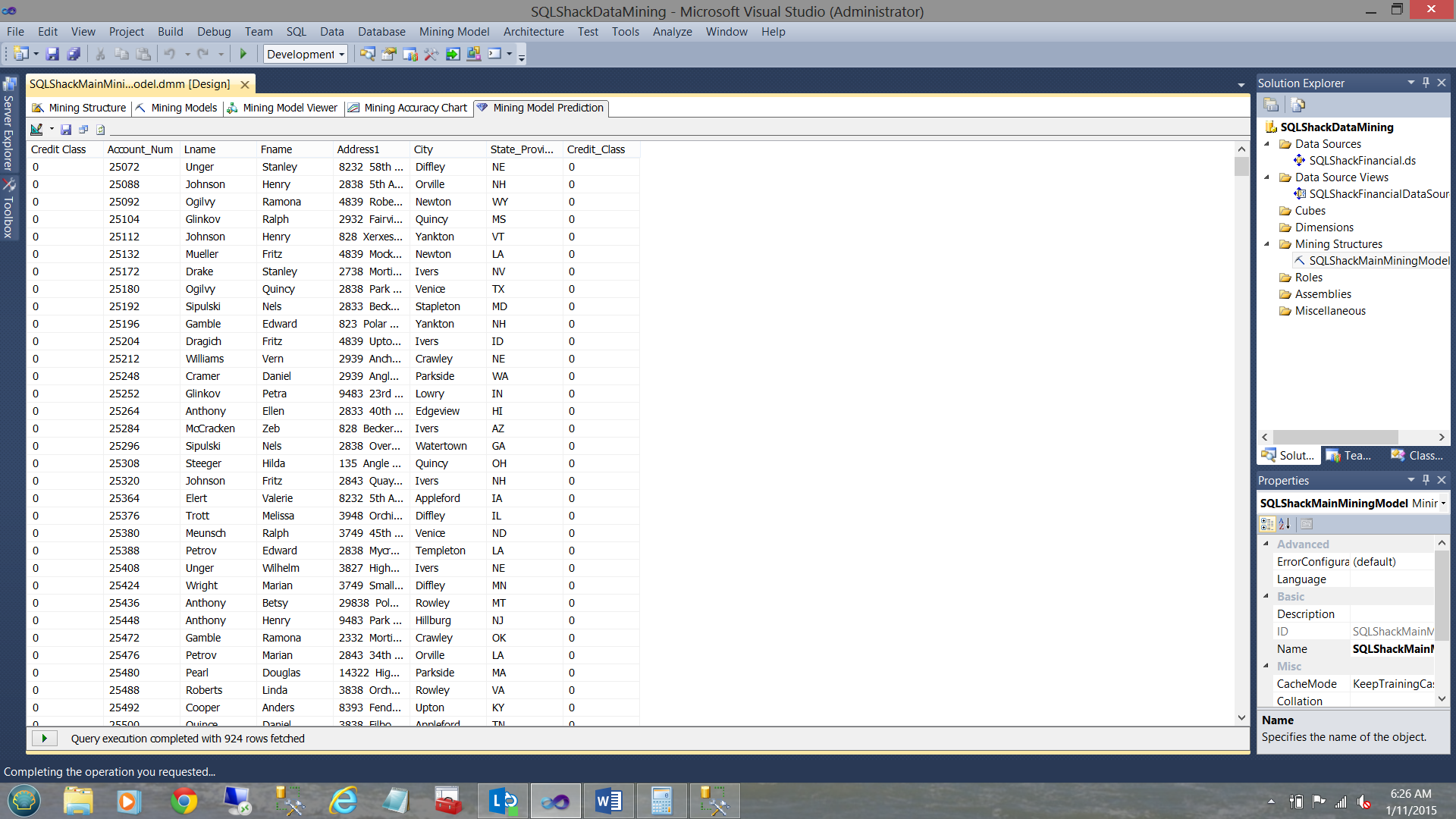
924 rows are returned which indicates a 95% accuracy. The only one take away from this 95% is that we are still on track with our model.. nothing more, nothing less.
Conclusions (if any)
It cannot be stressed enough that data mining is an iterative process. In real life business scenarios, one would take into consideration more degrees of freedom.
Attributes such as
- Salary
- Length of time at current job
- Age
- References (on a numeric scale 0 = bad 5 = great)
Etc.
Further, time must be spent in refining the actual combinations of these parameters with the myriad of mining models in order to ensure we are utilizing the most effective model(s).
In short, it is a trial and error exercise. The more data that we have and the more degrees of freedom that we utilize, the closer we come to the ‘truth’ and ‘reality’.
In the second part of this article (to be published soon), we shall see how we may utilize the information emanating from the models, in our day to day reporting activities.
Lastly, common sense and understanding are prerequisites to any successful data mining project. There are no correct answers, merely close approximates. This is the reality! Happy programming!
Steve has presented papers at 8 PASS Summits and one at PASS Europe 2009 and 2010. He has recently presented a Master Data Services presentation at the PASS Amsterdam Rally.
Steve has presented 5 papers at the Information Builders' Summits. He is a PASS regional mentor.
View all posts by Steve Simon
- Reporting in SQL Server – Using calculated Expressions within reports - December 19, 2016
- How to use Expressions within SQL Server Reporting Services to create efficient reports - December 9, 2016
- How to use SQL Server Data Quality Services to ensure the correct aggregation of data - November 9, 2016