In this article, in the series, we’ll discuss understanding and preparing data by using SQL unpivot.

As I announced in my previous article, Data science in SQL Server: pivoting and transposing data, this one is talking about the opposite process to pivoting, the unpivoting process. With unpivoting, you rotate the data to get rows from specific number of columns, with the original column names stored as a value in the rows of a new, unpivoted column. Unpivoting might be even more frequent operation in data science data preparation than pivoting because quite a lot of data exist in spreadsheets and other table formats that are not suitable for an immediate use.

Instead of any further explanation of unpivoting, I will show you the process through examples.

T-SQL Unpivot Operator and Other Possibilities

As always, I need some data to work on. The following query creates a table with pivoted data.

The following query checks the content of the table I just created.

Here is the result, the pivoted table:

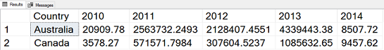
In a data science projects, you might have a task to forecast the sales over countries and years. You need to create time series, with years as time points. Since you have data for five years in five columns, you need to create five rows for each year. You will get five rows per country, with a new column that denotes the year, with the original column names [2010] to [2014] as the values of this new column. You will get another new column with sales data. The values of this column will be the respective values of the cells in the intersection of each country with each year. For example, the for the row with country Australia and year 2010, the sales value will be 20,909.78. My first query uses the T-SQL UNPIVOT operator.

Here is the unpivoted result. You can see that I used the name CYear for the year column (denoting calendar year) and Sales for the value column:

Similarly like the PIVOT operator, the UNPIVOT operator is also not a part of the ANSI SQL standard. In order to have your data science project code prepared for multiple database management systems, you might want to use the standard ANSI SQL expressions only. For each original row, for each country, you have to create five rows, one for each year. You can do it with a cross join of the original table with the tabular expression in the FROM clause that returns the five rows. Then you use the CASE expression to extract the correct value for each year. Finally, you need to eliminate rows with unknown sales. This last task is just to have completely the same logic as the PIVOT operator, which eliminates rows with NULLs in the value column. In your data science project, you might keep NULLs, and replace them with some default value, in order to have all time points present. Note that in the demo dataset I am using, there are no NULLs, so the result of the following query would be the same even without the WHERE clause.

In T-SQL, you could also use the CROSS APPLY operator to apply a tabular expression for each row from the original table. You can also create the five rows, one for each year, with the VALUES clause, which is a shorthand for multiple SELECT … UNION clauses. Like the following example shows, the query becomes shorter.

However, the APPLY operator is also a T-SQL extension of the ANSI standard. You might still prefer to use the standard SQL in your projects.

In all of the queries so far, I had to write manually the list of the values for the CYear column. Therefore, you can unpivot only a fixed number of original columns. The question is, of course, can you create this list dynamically, as I have shown in my previous article for the PIVOT operator. And the answer is yes. All you need to know is that in SQL Server, you can find all column names of all tables in sys.columns catalog view. Then you can use the STRING_AGG() function to get a delimited list of the column names.

It is time to switch to the languages that are more oriented towards data science.

Unpivoting in R

Let me read the pivoted data from SQL Server in R.

You can use the stack() function from the basic installation to unpivot the data. The following code stacks vertically the data from the SGY data frame without the first column.

Here is the result:

You can see that I lost the country values. I can add them back with the following code.

In the previous code, I used the rbind() function to multiply the first two rows of the original data frame with the first column only, with the country only. Now I have ten rows, which I can bind as a new column with the cbind() function to the result of the stack() function. Here is the result: Countryvaluesind 1Australia20909.782010 2Canada3578.272010 3 Australia 2563732.252011 4 Canada 571571.802011 5 Australia 2128407.462012 6 Canada 307604.522012 7 Australia 4339443.382013 8 Canada 1085632.652013 9 Australia 8507.722014 10 Canada 9457.622014

This was not a very useful code. Besides adding the countries manually, I also did not change the default column names for the two new columns, the values and the column.

To make the complete unpivoting dynamically, I can use the melt() function from the reshape package. Here is an example.

The following result shows that I still have default names for them to new columns. The melt() function assigns the names variable and value. In addition, I didn’t care about the order of the rows.

I will take care of the column names and the row order with the rename() and arrange() functions from the dplyr package.

Now I got the result I wanted.

I will show one more option in R – the gather() function from the tidyr package. I can define the new column names when calling this function directly. Then I can use the arrange() function again to sort the data, like the following code shows. The result is the same as above.

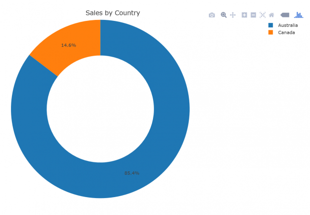
Time to show another graph. This time, I am using the plot_ly() function from the plotly library. With this library, you can make interactive graphs online. Therefore, the next graph opens in a Web browser.

Here is the plotly graph, showing the sales oved countries in a donut chart:

In the next section, I will show how to do the unpivoting in Python.

Python Pandas Unpivoting

Let me again start with imports and with reading the data from SQL Server.

I will find all methods I need for unpivoting in the pandas library. The first method I am showing is the unstack() method.

Here is the result:

I got a two-level index or a multi-index. I can use the rest_index() method to get flattened index structure with both levels shown explicitly, like the following code shows.

Here is the result:

Still, the result is not very useful. The melt() function returns a more standard data frame result.

You can see the output of the melt() function bellow:

Finally, let me also rename the columns and sort the data.

The next result is again in the form I wanted to achieve.

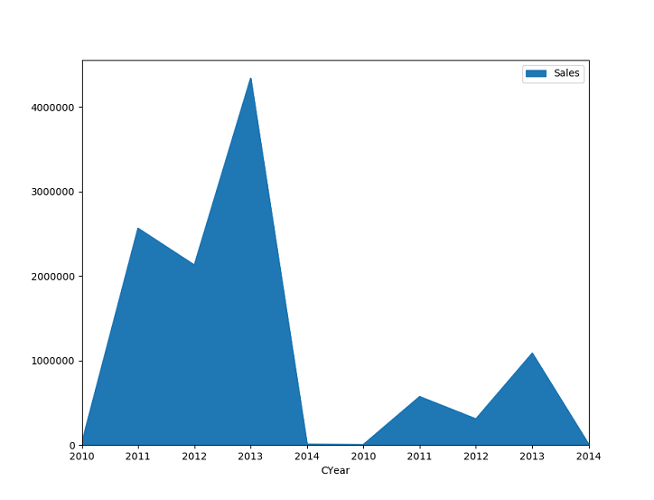
And for the last thing, let me show the sales over years for both countries together in a pandas area chart.

The following figure shows the graph:

Conclusion

I am done with pivoting and unpivoting. However, I am not done with the data preparation yet. So far, I always had a dataset with known values only. What happens if there are NULLs in the data? Stay tuned for the forthcoming articles.

Table of contents

Downloads

• Data Science in SQL Server Unpivoting Data_Code
• Data Science in SQL Server Unpivoting Data_Figures

• Author
• Recent Posts

Dejan Sarka

Dejan Sarka, MCT and Data Platform MVP, is an independent trainer and consultant that focuses on development of database & business intelligence applications.Besides projects, he spends about half of the time on training and mentoring. He is the founder of the Slovenian SQL Server and .NET Users Group. Dejan Sarka is the main author or coauthor of sixteen books about databases and SQL Server. He also developed many courses and seminars for Microsoft, SolidQ and Pluralsight.

View all posts by Dejan Sarka

Latest posts by Dejan Sarka (see all)

• Data Science in SQL Server: Unpivoting Data - October 29, 2018
• Data science in SQL Server: Data analysis and transformation – Using SQL pivot and transpose - October 11, 2018
• Data science in SQL Server: Data analysis and transformation – grouping and aggregating data II - September 28, 2018