
In my previous four articles, I worked on a single variable of a dataset. I have shown example code in T-SQL, R, and Python languages. I always used the same dataset. Therefore, you might have gotten the impression that in R and in Python, you can operate on a dataset the same way like you operate on an SQL Server table. However, there is a big difference between an SQL Server table and Python or R data frame.
In this article, will do a bit more formal introduction to R and Python data frames. I will show how to make basic operations on data frames, like filter them, make a projection, join and bind them, and sort them. For the sake of completeness, I am starting with T-SQL. Of course, the first part is really just a very brief recapitulation of the basic SELECT statement.
Core T-SQL SELECT statement elements
The simplest query to retrieve the data you can write includes the SELECT and the FROM clauses. In the select clause, you can use the star character, literally SELECT *, to denote that you need all columns from a table in the result set.
Better than using SELECT * is to explicitly list only the columns you need. This means you are returning only a projection on the table. A projection means you filter the columns. Of course, you can filter also the rows with the WHERE clause.
In a relational database, you typically have data spread in multiple tables. Each table represents a set of entities of the same kind, like customers, or products, or orders. In order to get result sets meaningful for the business your database supports, you most of the time need to retrieve data from multiple tables in the same query. You need to join two or more tables based on some conditions. The most frequent kind of a join is the inner join. Rows returned are those for which the condition in the join predicate for the two tables joined evaluates to true. Note that in a relational database, you have three-valued logic, because there is always a possibility that a piece of data is unknown. You mark the unknown with the NULL keyword. A predicate can thus evaluate to true, false or NULL. For an inner join, the order of the tables involved in the join is not important.
In the query where you join multiple tables, you should use table aliases. If a column’s name is unique across all tables in the query, then you can use it without table name. You can shorten the two-part column names by using table aliases. You specify table aliases in the FROM clause. Once you specify table aliases, you must always use the aliases; you can’t refer to the original table names in that query anymore. Please note that a column name might be unique in the query at the moment when you write the query. However, later somebody could add a column with the same name in another table involved in the query. If the column name is not preceded by an alias or by the table name, you would get an error when executing the query because of the ambiguous column name. In order to make the code more stable and more readable, you should always use table aliases for each column in the query. You can specify column aliases as well.
A table in SQL Server represents a set. In a set, the order of the elements is not defined. Therefore, you cannot refer to a row or a column in a table by position. Also, the result of the SELECT statement does not guarantee any specific ordering. If you want to return the data in a specific order, you need to use the ORDER BY clause. The following query shows these basic SELECT elements.
|
1 2 3 4 5 6 7 8 9 10 |
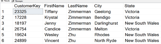
USE AdventureWorksDW2016; GO -- Basic SELECT statement elements SELECT c.CustomerKey, c.FirstName, c.LastName, g.City, g.StateProvinceName AS State FROM dbo.DimCustomer AS c INNER JOIN dbo.DimGeography AS g ON c.GeographyKey = g.GeographyKey WHERE g.EnglishCountryRegionName = N'Australia' ORDER BY c.LastName DESC, c.FirstName DESC; |
The following figure shows the partial results, limited to the first six rows only. Please note the order of the rows and other elements of the basic SELECT statement implemented.
R data frame
In R, you operate on matrices, not on tables. A matrix is a two-dimensional array of values of the same type. The elements are ordered, and you can refer to them by position.
The most important data structure in R is a data frame. Most of the time, you analyze data stored in a data frame. Data frames are matrices where each variable can be of a different type. Remember, a variable is stored in a column, and all values of a single variable must be of the same type. Data frames are very similar to SQL Server tables. However, they are still matrices, meaning that you can refer to the elements by position and that they are ordered.
Most of the times, you get a data frame from your data source, for example from a SQL Server database. You can also enter the data manually, or read it from many other sources, including text files, Excel, and many more. The following code reads the data from SQL Server AdventureWorksDW2016 demo database, the dbo.vTargetMail view.
|
1 2 3 4 5 6 7 8 |
library(RODBC) # Connecting and reading the data con <- odbcConnect("AWDW", uid = "RUser", pwd = "Pa$$w0rd") TM <- as.data.frame(sqlQuery(con, "SELECT CustomerKey, MaritalStatus, Gender, Age FROM dbo.vTargetMail;"), stringsAsFactors = TRUE) close(con) |
The following code shows how you can access the data in a data frame by the position or mixed by the position and column names. Please note that the index of the first row or column is 1, and that the boundaries are included – you get three rows and two columns.
|
1 2 |
TM[1:3, 1:2]; TM[1:3, c("MaritalStatus", "Gender")]; |
The result of the previous two rows is the same:
| CustomerKey | MaritalStatus | |
| 1 | 11000 | M |
| 2 | 11001 | S |
| 3 | 11002 | M |
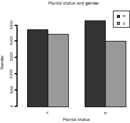
You can refer to columns similarly like you refer to them in T-SQL, where you use table.column dotation; in R, the dollar sign replaces the dot, and therefore you refer to columns with dataframe$column. The following code shows how to refer to the columns. It does the crosstabulation of the MaritalStatus and Gender columns and shows this in a bar chart.
|
1 2 3 4 5 6 7 8 9 |
# $ Notation mg <- table(TM$MaritalStatus, TM$Gender); mg barplot(mg, main = 'Marital status and gender', xlab = 'MaritalStatus', ylab = 'Gender', col = c("blue", "yellow"), beside = TRUE, legend = TRUE) |
Here is the bar chart.
For a projection, you simply select appropriate columns, like the following code shows. It creates two new data frames with subset of the columns only.
|
1 2 3 4 5 6 7 |
# Projections cols1 <- c("CustomerKey", "MaritalStatus") TM1 <- TM[cols1] cols2 <- c("CustomerKey", "Gender") TM2 <- TM[cols2] TM1[1:3, 1:2] TM2[1:3, 1:2] |
Here are the first three rows of the two new data frames.
| CustomerKey | MaritalStatus | |
| 1 | 11000 | M |
| 2 | 11001 | S |
| 3 | 11002 | M |
| CustomerKey | Gender | |
| 1 | 11000 | M |
| 2 | 11001 | M |
| 3 | 11002 | M |
You can merge two data frames using some column values from a column that appears in both of them. This is very similar to T-SQL join. The following code performs the merge of the two previously created data frames.
|
1 2 3 |
# Merge datasets TM3 <- merge(TM1, TM2, by = "CustomerKey") TM3[1:3, 1:3] |
The results are:
| CustomerKey | MaritalStatus | Gender | |
| 1 | 11000 | M | M |
| 2 | 11001 | S | M |
| 3 | 11002 | M | M |
However, data frames are ordered. You can rely on the order, unless you reorder a data frame, of course. Since I created the two projection data frames TM1 and TM2 from the original TM data frame without reordering them, they maintain the original order. Instead of joining them, I can simply bind the columns, row by row, by the cbind() function, like the following code shows.
|
1 2 3 |
# Binding datasets TM4 <- cbind(TM1, TM2) TM4[1:3, 1:4] |
Note the results:
| CustomerKey | MaritalStatus | CustomerKey.1 | Gender | |
| 1 | 11000 | M | 11000 | M |
| 2 | 11001 | S | 11001 | M |
| 3 | 11002 | M | 11002 | M |
The CustomerKey column is listed twice, and the second time it is automatically renamed.
You can filter a data frame by using a predicate when you refer to the index of rows or columns. The following code creates a two new data frames with the same columns, CustomerKey and MaritalStatus. The first data frame is filtered to include only two customers with the lowest CustomerKey, and the second includes only two customers with the highest CustomerKey values. Both data frames have the same columns. You can bind such data frames by rows with the rbind() function. This is a similar process like the UNION ALL clause does in T-SQL.
|
1 2 3 4 5 |
# Filtering and row binding data TM1 <- TM[TM$CustomerKey < 11002, cols1] TM2 <- TM[TM$CustomerKey > 29481, cols1] TM5 <- rbind(TM1, TM2) TM5 |
Here is the content of complete TM5 data fame.
| CustomerKey | MaritalStatus | |
| 1 | 11000 | M |
| 2 | 11001 | S |
| 18483 | 29482 | M |
| 18484 | 29483 | M |
Finally, you can reorder a data frame by using the order() function in the index reference. The following code creates a reordered data frame by sorting the rows over the Age column. Note the minus sign in the order() function – it means sort descending.
|
1 2 3 |
# Sort TMSortedByAge <- TM[order(-TM$Age), c("CustomerKey", "Age")] TMSortedByAge[1:5, 1:2] |
So here are the reordered first five rows.
| CustomerKey | Age | |
| 1726 | 12725 | 99 |
| 5456 | 16455 | 98 |
| 3842 | 14841 | 97 |
| 3993 | 14992 | 97 |
| 7035 | 18034 | 97 |
Python Pandas data frame
In Python, there is also the data frame object, like in R. However, it is not part of the basic engine like in R. It is defined in the pandas library. You can communicate with SQL Server through the pandas data frames. But before getting there, you need first to refer to the numpy library, which brings efficient work with matrices to Python. The following code does the necessary imports and reads the data from SQL Server.
|
1 2 3 4 5 6 7 8 9 |
import numpy as np import pandas as pd import pyodbc import matplotlib.pyplot as plt # Connecting and reading the data con = pyodbc.connect('DSN=AWDW;UID=RUser;PWD=Pa$$w0rd') query = """SELECT CustomerKey, MaritalStatus, Gender, Age FROM dbo.vTargetMail;""" TM = pd.read_sql(query, con) |
The pandas data frame has many built methods for which you need separate functions in R. For example, you can use the pandas crosstab() function to cross tabulate the data like the R table() function. However, you don’t need a separate function to plot the data; you ca use the pandas data frame plot() function, like the following code shows.
|
1 2 3 4 5 6 7 8 |
# A graph of marital status and gender pd.crosstab(TM.MaritalStatus + TM.Gender, columns = 'Count', rownames = 'X').plot(kind = 'barh', legend = False, title = 'Marital status and gender', fontsize = 12) plt.show() |
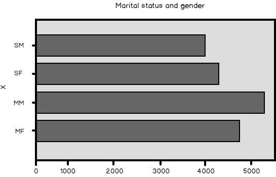
Not that the result of the pandas crosstab() function is a new data frame, and I am calling the plot() method of this data frame in order to produce this time a horizontal bar chart, like you can see in the following figure.

You make a projection of a data frame by selecting a subset of columns listed by their names in an array, like the following code shows.
|
1 2 3 |
# Projections TM1 = TM[["CustomerKey", "MaritalStatus"]] TM2 = TM[["CustomerKey", "Gender"]] |
I created two new data frames in the previous code. Because a data frame is a matrix in Python as well, I can refer to the elements by their positional index with the iloc(), or index locate method:
|
1 2 3 |
# Positional access TM1.iloc[0:3, 0:2] TM2.iloc[0:3, 0:2] |
Note that the index is zero-based. But there is another interesting difference from R. Please observe the results of the previous code.
| CustomerKey | MaritalStatus | |
| 0 | 11000 | M |
| 1 | 11001 | S |
| 2 | 11002 | M |
| CustomerKey | Gender | |
| 0 | 11000 | M |
| 1 | 11001 | M |
| 2 | 11002 | M |
Not that when you refer to the elements of a data frame by the index position, the upper boundary is not included. For example, the fourth row (index value 3) is not included in any of the results.
With the loc() method you can locate the elements based on a predicate for the rows and columns. For example, the following code selects Only rows where Age is greater than 97 and lists the three columns included in the results explicitly in an array.
|
1 2 |
# Filter and projection TM.loc[TM.Age > 97, ["CustomerKey", "Age", "Gender"]] |
| CustomerKey | Age | Gender | |
| 1725 | 12725 | 99 | F |
| 5455 | 16455 | 98 | F |
In order to join two data frames, you can use the merge() pandas function, and specify the column you want to use for the join. This is similar to R merge() function. You can see this process in the following code.
|
1 2 3 |
# Joining data frames TM3 = pd.merge(TM1, TM2, on = "CustomerKey") TM3.iloc[0:3, 0:3] |
The first three rows of the merged data frame are shown below.
| CustomerKey | MaritalStatus | Gender | |
| 0 | 11000 | M | M |
| 1 | 11001 | S | M |
| 2 | 11002 | M | M |
Finally, you can reorder a data frame with help of the sort() method, like shown in the following code.
|
1 2 3 |
# Sort TMSortedByAge = TM.sort(["Age"], ascending = False) TMSortedByAge.iloc[0:5, 0:4] |
And here is the last result in this article.
| CustomerKey | MaritalStatus | Gender | Age | |
| 1725 | 12725 | M | F | 99 |
| 5455 | 16455 | M | F | 98 |
| 3841 | 14841 | M | M | 97 |
| 7034 | 18034 | M | M | 97 |
| 3992 | 14992 | M | M | 97 |
Conclusion
In this article, you learned how to do the basic operations on a whole dataset. For the next article, I plan to show how you can do more advanced operations, like grouping and aggregating data in t-SQL, R, and Python.
Table of contents
References

View all posts by Dejan Sarka
- Data Science in SQL Server: Unpivoting Data - October 29, 2018
- Data science in SQL Server: Data analysis and transformation – Using SQL pivot and transpose - October 11, 2018
- Data science in SQL Server: Data analysis and transformation – grouping and aggregating data II - September 28, 2018