

I started to explain the data preparation part of a data science project with discrete variables. As you should know by now, discrete variables can be categorical or ordinal. For ordinal, you have to define the order either through the values of the variable or inform about the order the R or the Python execution engine. Let me start this article with Python code that shows another way how to define the order of the Education variable from the dbo.vTargetMail view from the AdventureWorksDW2016 demo database.
|
1 2 3 4 5 6 7 8 9 10 11 12 13 14 15 16 17 18 19 20 21 22 23 24 25 26 |
# Imports needed import numpy as np import pandas as pd import pyodbc import matplotlib.pyplot as plt import seaborn as sns # Connecting and reading the Education con = pyodbc.connect('DSN=AWDW;UID=RUser;PWD=Pa$$w0rd') query = """SELECT CustomerKey, EnglishEducation AS Education FROM dbo.vTargetMail;""" TM = pd.read_sql(query, con) # Define Education as categorical TM['Education'] = TM['Education'].astype('category') # Reordering Education TM['Education'].cat.reorder_categories( ["Partial High School", "High School","Partial College", "Bachelors", "Graduate Degree"], inplace=True) TM['Education'] TM['Education'].value_counts(sort = False) # Education barchart sns.countplot(x="Education", data=TM); plt.show() |
This code imports the necessary libraries, reads the data from SQL Server, defines Education as categorical, and then reorder the values using the pandas built-in function cat.reorder_categories(). Then the code shows the distribution of the values and the bar plot for this variable. For the sake of brevity, I am not showing the bar chart, because it is the same as I have shown in my previous article, Data science, data understanding and preparation – ordinal variables and dummies.
Some data science algorithms need only discrete variables for the input. If you have a continuous variable, you have to group or bin the values. Sometimes you want to bin a continuous variable for other reasons as well, for example, to show the distribution in a bar chart, or to use it for grouping and pivoting. Therefore, let me explain a couple of options you have for binning a continuous variable.
Equal width binning
There are many ways to do the binning. I will introduce here the three most popular ones, the equal width, equal height, and custom binning. Let me start with T-SQL code that prepares a new table with the Age variable and the key, Age lowered for 10 years, to make the data more plausible.
|
1 2 3 4 5 6 7 8 9 10 11 12 13 14 15 16 17 18 |
USE AdventureWorksDW2016; GO -- Preparing demo table for the continuous variable DROP TABLE IF EXISTS dbo.TMAge; GO SELECT CustomerKey, Age-10 AS Age INTO dbo.TMAge FROM dbo.vTargetMail; GO -- Data overview SELECT MIN(Age) AS minA, MAX(Age) AS maxA, MAX(Age) - MIN(Age) AS rngA, AVG(Age) AS avgA, 1.0 * (MAX(Age) - MIN(Age)) / 5 AS binwidth FROM dbo.TMAge; |
Here are the results.
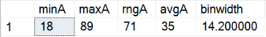
You can see the minimal, maximal and average value of the age, the range, and the width of a bin for equal width binning. Equal width binning means that the width of each bin is equal, no matter of the number of cases in each bin. This kind of binning preserves well the distribution of the continuous variable, especially if the number of bins is high. The following Python code reads the Age from the table just created, and then bins it into 20 equal width bins, and then creates the bar chart.
|
1 2 3 4 5 6 7 8 9 10 11 12 13 14 |
# Connecting and reading the Age con = pyodbc.connect('DSN=AWDW;UID=RUser;PWD=Pa$$w0rd') query = """SELECT CustomerKey, Age FROM dbo.TMAge;""" TMAge = pd.read_sql(query, con) # Show the Age continuous variable in 20 equal width bins TMAge['AgeEWB'] = pd.cut(TMAge['Age'], 20) TMAge['AgeEWB'].value_counts() pd.crosstab(TMAge.AgeEWB, columns = 'Count').plot(kind = 'bar', legend = False, title = 'AgeEWB') plt.show() |
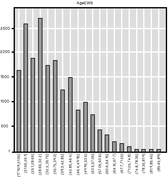
So here is the bar chart. You can see the distribution of Age quite well.
If you use less bins, then the bar chart follows the shape of the distribution worse. The next Python code bins the values of the Age in 5 bins.
|
1 2 3 |
# Equal width binning - 5 bins TMAge['AgeEWB'] = pd.cut(TMAge['Age'], 5) TMAge['AgeEWB'].value_counts(sort = False) |
These are the counts, or the frequency distribution of the Age, binned in 5 equal width bins.

In R, you can use the cut() function from the basic installation, without any additional package, to bin the data. The following code loads the RODBC library, reads the SQL Server table, and then bins the continuous variable, Age, in 5 equal width bins. The counts, the result of the table() function, is the same as the result from the Python code.
|
1 2 3 4 5 6 7 8 9 10 11 12 13 14 15 |
# Load RODBC library (install only if needed) # install.packages("RODBC") library(RODBC) # Connecting and reading the data con <- odbcConnect("AWDW", uid = "RUser", pwd = "Pa$$w0rd") TMAge <- as.data.frame(sqlQuery(con, "SELECT CustomerKey, Age FROM dbo.TMAge;"), stringsAsFactors = TRUE) close(con) # Equal width binning of a continuous variable TMAge["AgeEWB"] = cut(TMAge$Age, 5) table(TMAge$AgeEWB) |
Finally, let’s do the equal width binning in T-SQL. The code first reads the minimal and the maximal value of Age and calculated the width of the bins, considering binning into 5 bins. Then the next query uses the CASE clause to define the bins and the labels of the bins.
|
1 2 3 4 5 6 7 8 9 10 11 12 13 14 15 16 17 18 19 20 21 22 23 24 25 |
-- Equal width binning of a continuous variable DECLARE @binwidth AS NUMERIC(5,2), @minA AS INT, @maxA AS INT; SELECT @minA = MIN(AGE), @maxa = MAX(Age), @binwidth = 1.0 * (MAX(Age) - MIN(Age)) / 5 FROM dbo.TMAge; SELECT CustomerKey, Age, CASE WHEN Age >= @minA + 0 * @binwidth AND Age < @minA + 1 * @binwidth THEN CAST((@minA + 0 * @binwidth) AS VARCHAR(5)) + ' - ' + CAST((@minA + 1 * @binwidth) AS VARCHAR(5)) WHEN Age >= @minA + 1 * @binwidth AND Age < @minA + 2 * @binwidth THEN CAST((@minA + 1 * @binwidth) AS VARCHAR(5)) + ' - ' + CAST((@minA + 2 * @binwidth) AS VARCHAR(5)) WHEN Age >= @minA + 2 * @binwidth AND Age < @minA + 3 * @binwidth THEN CAST((@minA + 2 * @binwidth) AS VARCHAR(5)) + ' - ' + CAST((@minA + 3 * @binwidth) AS VARCHAR(5)) WHEN Age >= @minA + 3 * @binwidth AND Age < @minA + 4 * @binwidth THEN CAST((@minA + 3 * @binwidth) AS VARCHAR(5)) + ' - ' + CAST((@minA + 4 * @binwidth) AS VARCHAR(5)) ELSE CAST((@minA + 4 * @binwidth) AS VARCHAR(5)) + ' + ' END AS AgeEWB FROM dbo.TMAge; GO |
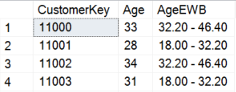
Again, the distribution of the binned continuous variable is the same as in Python or R. Here are the partial results of the query, showing a couple of rows with the original and the binned values of the Age continuous variable.
Equal height binning
Equal height binning of a continuous variable means that after the binning, there is am approximately equal number of cases in each bin, and the width of the bins varies. You can do this very simply with the T_SQL NTILE() function, like the following code shows. Note that I used the ORDER BY clause only to shuffle the results, to get all possible tiles of the continuous variable in the first few rows.
|
1 2 3 4 5 6 7 |
-- Equal height binning SELECT CustomerKey, Age, CAST(NTILE(5) OVER(ORDER BY Age) AS CHAR(1)) AS AgeEHB FROM dbo.TMAge ORDER BY NEWID(); GO |
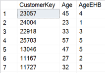
Here are partial results.
In R, I will create a function for the equal height binning. Let me develop the function step by step. First, I use the integer division to calculate the minimal number of cases in each bin for 5 bins.
|
1 2 |
# Lower limit for the number of cases in a bin length(TMAge$Age) %/% 5 |
The number given is 3,696. If the number of cases would be divisible by 5, then each bin would have this number of cases. Let’s create a vector with five times this number.
|
1 2 |
# Create the vector of the bins with number of cases rep(length(TMAge$Age) %/% 5, 5) |
However, the number of cases in this data frame we are using is not divisible by 5. With the modulo operator, you can see that there is a remainder of 4 rows.
|
1 2 |
# How many bins need a case more length(TMAge$Age) %% 5 |
We will add these four cases to the first four bins, like does the NTILE() function in T-SQL. The following code creates a vector of five values, namely (1, 1, 1, 1, 0), which will be added to the number of cases in each bin.
|
1 2 |
# Array to add cases to the first 4 bins ifelse(1:5 <= length(TMAge$Age) %% 5, 1, 0) |
Finally, here is the code that creates the binning function and does the binning.
|
1 2 3 4 5 6 7 8 9 10 |
# Equal height binning - a function EHBinning <- function(data, nofbins) { bincases <- rep(length(data) %/% nofbins, nofbins) bincases <- bincases + ifelse(1:nofbins <= length(data) %% nofbins, 1, 0) bin <- rep(1:nofbins, bincases) bin <- bin[rank(data, ties.method = "last")] return(factor(bin, levels = 1:nofbins, ordered = TRUE)) } TMAge["AgeEHB"] = EHBinning(TMAge$Age, 5) table(TMAge$AgeEHB) |
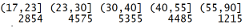
The table() function shows the number of cases in each bin, 3697, 3697, 3697, 3697, and 3696.
In Python, you can use the pandas qcut() function for the equal height, or quantile binning, like the following code shows.
|
1 2 3 |
# Equal height binning TMAge['AgeEHB'] = pd.qcut(TMAge['Age'], 5) TMAge['AgeEHB'].value_counts(sort = False) |
Note the results – the distribution of the values slightly differs from the results of the T-SQL and R code.
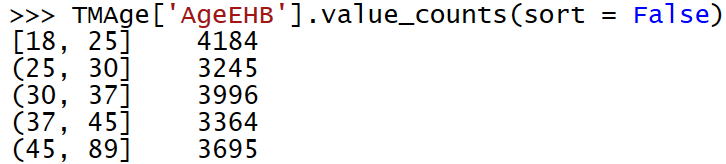
These small differences are due to the fact that the qcut() function classifies all cases with the same value in a single tile. In Python, all cases with Age of 25 are in the first tile; in T-SQL and R, some of these cases were assigned to tile 2, in order to have a really equal number of cases in each tile. Nevertheless, these differences are small and not really important.
Custom binning
If you want to follow the real life or business logic, you need to do a custom binning. The Age continuous variable is a very nice example. Age is many times binned with a custom logic. You can imagine that one-year difference in age means much more when you are a teenager than when you are in sixties or seventies. Therefore, you create narrower bins for the smaller values and wider for the bigger values of the Age continuous variable. Here is the T-SQL code that does the custom binning.
|
1 2 3 4 5 6 7 8 9 10 11 12 13 14 15 |
-- Custom binning SELECT CustomerKey, Age, CASE WHEN Age >= 18 AND Age < 24 THEN '18 - 23' WHEN Age >= 24 AND Age < 31 THEN '24 - 30' WHEN Age >= 31 AND Age < 41 THEN '31 - 40' WHEN Age >= 41 AND Age < 56 THEN '41 - 55' ELSE '56 +' END AS AgeCUB FROM dbo.TMAge; GO |
You can do it easily with the pandas cut() function in Python as well. You only need to provide the function a vector with the cutting values.
|
1 2 3 4 5 6 7 8 9 10 |
# Custom binning custombins = [17, 23, 30, 40, 55, 90] pd.cut(TMAge['Age'], custombins) TMAge['AgeCUB'] = pd.cut(TMAge['Age'], custombins) TMAge['AgeCUB'].value_counts(sort = False) pd.crosstab(TMAge.AgeCUB, columns = 'Count').plot(kind = 'bar', legend = False, title = 'AgeCUB') plt.show() |
Here is the graph showing the distribution of the Age binned in custom bins.

Finally, let’s do the custom binning in R. I am using the cut() function again and feed it with a vector of the cutting points, like in Python.
|
1 2 3 |
# Custom binning TMAge["AgeCUB"] = cut(TMAge$Age, c(17, 23, 30, 40, 55, 90)) table(TMAge$AgeCUB) |
And here are the counts of the binned continuous variable.
Conclusion
In Data science working with variables is commonplace. Equal width and custom binning are both quite intuitive techniques for managing continuous variables. You can ask yourself why you would use equal height binning. Of course, there is a reason for this kind of binning as well. You preserve more information with equal height binning than with other two options when working with a continuous variable. I will explain this in detail in my next article in this data science series.
Table of contents
References

View all posts by Dejan Sarka
- Data Science in SQL Server: Unpivoting Data - October 29, 2018
- Data science in SQL Server: Data analysis and transformation – Using SQL pivot and transpose - October 11, 2018
- Data science in SQL Server: Data analysis and transformation – grouping and aggregating data II - September 28, 2018