

Data science, machine learning, data mining, advanced analytics, or however you want to name it, is a hot topic these days. Many people would like to start some project in this area. However, very soon after the start you realize you have a huge problem: your data. Your data might come from your line of business applications, data warehouses, or even external sources. Typically, it is not prepared for applying advanced analytical algorithms on it straight out of the source. In addition, you have to understand your data thoroughly, otherwise you might feed the algorithms with inappropriate variables. Soon you learn the fact that is well known to seasoned data scientists: you spend around 70-80% of the time dedicated to a data science project on data preparation and understanding.
Note: To learn more about data preparation, please read Different Stakeholders, Different Views: Why Database Management Requires a Systematic Approach article.
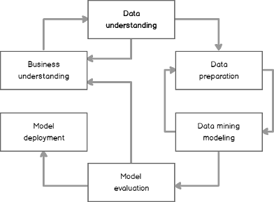
The whole data science project lifecycle is described with cross-industry standard process for data mining, by acronym CRISP-DM, described well in a Wikipedia article, which you can access by using this link. The following figure shows the process graphically.
With this article, I am starting a series of articles on exactly these two issues, data understanding and data preparation. I will explain the problems and show the solutions in different programming languages, including T-SQL, R, and Python. I hope that you will find these articles valuable in your data science routines.
Datasets, cases and variables
As I mentioned, I will focus on the data understanding and preparation part only. But don’t forget that you need to have a god business problem understanding as well. By understanding your business problem, you can also understand the data much better. In data science, you analyze datasets that consist of cases, which are described by their variables. If you are working with SQL Server, then a dataset is represented by a table, where a case is a row and a variable is a column. In R and Python, you use the data frame objects to represent datasets to analyze. Data frames look like tables; however, they are matrices. This means that you can access the data positionally.
The first issue you got is how to define a case. Sometimes it’s not so simple as you imagine. Let’s say that you need to analyze phone calls within a family and compare them to the calls outside a family. In this example, you might decide that your case is a single person, or a single family. Anyway, you prepare a dataset, where you gather together all information about your case.
Ways to measure data values
Your variables can measure values in different ways. Discrete variables can take a value only from a limited pool of values. For example, you might have information about the relationship status of your customers. You track only if the customer is married or is engaged in any other kind of relationship or single. The relationship status variable could then occupy two states only: “single” and “engaged”. Such a variable is categorical, or also called nominal variable.
Discrete variables can also have intrinsic order. You can rank the values; however, you cannot use any arithmetic on the values. Such variables are called ranks, or also ordinal variables. Education is a good example. There is an order between different possible values, or levels, of education.
There are also some specific discrete variables. If a variable can take only a single value, meaning the variable is actually a constant, then it is not useful for analysis, and you can simply drop it from the dataset. If a variable can take a value from a pool limited to two values only, like the relationship status I mentioned above, then this is a dichotomous variable. If you represent the stated with numbers 0 and 1 or false and true, using either integer or bit data type, then this is a binary variable.
Variables can be also continuous, like numbers, or dates. Still, the pool of the possible values can be limited. Maybe you need to use the temperature of the air in your analysis. Of course, temperature is limited on the left side – it can’t go below absolute zero. Time intervals, like periods when somebody used a service, have a lower and an upper boundary. These variables are intervals. Arithmetic is many times somehow limited with such variables. Looking at the temperature example, subtraction of two temperatures might have sense, but addition not. You should check what arithmetic is allowed for every interval in your dataset.
The least amount of problems usually come with true numeric variables, which are continuous and not limited on any side. They usually allow any kind of arithmetic operation on them.
Continuous variables might have a very specific distribution. Of course, you are familiar with the identity property or with sequences in SQL Server. Identity columns’ values are ever-growing. Such variables are monotonic. They might still be useful for your analysis. For example, a higher identity value might tell you that the case was introduced in the dataset later than the one with a lower value. Again, you should understand how your data is collected. You know that it is possible to insert identity values also manually, although this is not a very frequent case. However, if you cannot rely on the monotonic behavior of your identity columns, they might not be quite useful for further analysis.
Overview of discrete variables
Overview of a variable actually means an overview of the variable’s distribution. You do this overview by using different kind of charts and descriptive statistics.
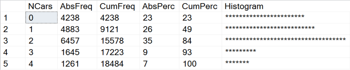
To see the distribution of discrete variables, you use frequency tables, or shortly frequencies. In a frequency table, you can show values, counts of those values, the percentage of the value count compared with the total count or the absolute percentage, the running total of the counts or the cumulative frequency, the running total of the percentages or the cumulative percent, and a bar char or a histogram of the counts.
The following code shows how you can create a frequency table with T-SQL. I am using the AdventureWorksDW2016 demo database, the dbo.vTargetMail view as the dataset, and analyze the NumberCarsOwned variable. You can download the backup of this database from GitHub.
|
1 2 3 4 5 6 7 8 9 10 11 12 13 14 15 16 17 18 19 20 21 22 23 24 25 |
USE AdventureWorksDW2016; GO WITH freqCTE AS ( SELECT v.NumberCarsOwned, COUNT(v.NumberCarsOwned) AS AbsFreq, CAST(ROUND(100. * (COUNT(v.NumberCarsOwned)) / (SELECT COUNT(*) FROM vTargetMail), 0) AS INT) AS AbsPerc FROM dbo.vTargetMail AS v GROUP BY v.NumberCarsOwned ) SELECT NumberCarsOwned AS NCars, AbsFreq, SUM(AbsFreq) OVER(ORDER BY NumberCarsOwned ROWS BETWEEN UNBOUNDED PRECEDING AND CURRENT ROW) AS CumFreq, AbsPerc, SUM(AbsPerc) OVER(ORDER BY NumberCarsOwned ROWS BETWEEN UNBOUNDED PRECEDING AND CURRENT ROW) AS CumPerc, CAST(REPLICATE('*',AbsPerc) AS VARCHAR(50)) AS Histogram FROM freqCTE ORDER BY NumberCarsOwned; |
The following figure shows the results of the previous query.
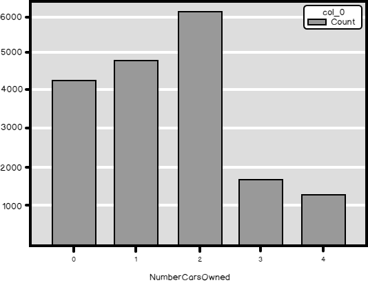
Of course, you can quickly do a similar overview with Python. If you are new to Python, I suggest you start with my introducing article about it, aimed at SQL Server specialists. You can execute this code in Visual Studio 2017. I explained the installation of SQL Server 2017 ML Services and Visual Studio 2017 for data science and analytical applications in the article I just mentioned. Here is the Python code.
|
1 2 3 4 5 6 7 8 9 10 11 12 13 14 15 16 |
# Imports needed import numpy as np import pandas as pd import pyodbc import matplotlib.pyplot as plt # Connecting and reading the data con = pyodbc.connect('DSN=AWDW;UID=RUser;PWD=********') query = """SELECT NumberCarsOwned FROM dbo.vTargetMail;""" TM = pd.read_sql(query, con) # Counts table and a bar chart pd.crosstab(TM.NumberCarsOwned, columns = 'Count') pd.crosstab(TM.NumberCarsOwned, columns = 'Count').plot(kind = 'bar') plt.show() |
This code produces the counts and also a nice graph, shown in the following figure.
Note that I used the ODBC Data Sources tool to create a system DSN called AWDW in advance. It points to my AdventureWorksDW2016 demo database. For the connection, I use the RUser SQL Server login I created specifically for Python and R. Of course, I created a database user in the AdventureWorksDW2016 database for this user and gave the user permission to read the data.
Finally, let me show you and example in R. If you are new to R, I suggest you download the slides and the demos from my Introducing R session I delivered at the SQL Saturday #626 Budapest event. You will get also the link you need to download the RStudio IDE development tool in this presentation if you prefer this tool to Visual Studio. Anyway, here is the R code.
|
1 2 3 4 5 6 7 8 9 10 11 12 13 14 15 16 |
# Install and load RODBC library install.packages("RODBC") library(RODBC) # Connecting and reading the data con <- odbcConnect("AWDW", uid = "RUser", pwd = "********") TM <- as.data.frame(sqlQuery(con, "SELECT NumberCarsOwned FROM dbo.vTargetMail;"), stringsAsFactors = TRUE) close(con) # Package descr install.packages("descr") library(descr) freq(TM$NumberCarsOwned, col = 'light blue') |
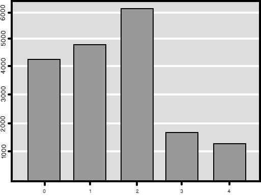
Note that in R, you typically need many additional packages. In this case, I used the descr package, which brings a lot of useful descriptive statistics functions. The freq() function I called returns a frequency table with counts and absolute percentages. In addition, it returns a graph, which you can see in the following figure.
Conclusion
This article is just a small teaser, a brief introduction of the big amount of work with data overview and preparation for data science projects. In my following articles, I intend to add quite a few more articles on this topic, with more advanced problems explained and resolved, and with more statistical procedures used for in-depth data understanding.
Table of contents
Downloads
References
- Introduction to Python
- Introduction to R
- Python Pandas.DataFrame
- R Tutorial: Data Frame
- The descr package documentation
- SELECT – OVER Clause (Transact-SQL)

View all posts by Dejan Sarka
- Data Science in SQL Server: Unpivoting Data - October 29, 2018
- Data science in SQL Server: Data analysis and transformation – Using SQL pivot and transpose - October 11, 2018
- Data science in SQL Server: Data analysis and transformation – grouping and aggregating data II - September 28, 2018