

Previously, in this Data science series, I already tacitly did quite a few aggregations over the whole dataset and aggregations over groups of data. Of course, the vast majority of the readers here is familiar with the GROUP BY clause in the T-SQL SELECT statement and with the basic aggregate functions. Therefore, in this article, I want to show some advanced aggregation options in T-SQL and grouping in aggregations of data in an R or a Python data frame.
Aggregating data might be a part of data preparation in data science, a part of data overview, or even already a part of the finaly analysis of the data.
T-SQL Grouping Sets
The T-SQL language does not have a plethora of different aggregate functions. However, you can do a lot of different ways of grouping of the same rows with just a few lines of code in T-SQL.
Let me start with the basic aggregation over groups in T-SQL. The following code calculates the number of customers per country ordered by the country name, using the COUNT(*) aggregate function. You define the grouping variables in the GROUP BY clause.
|
1 2 3 4 5 6 7 8 |
USE AdventureWorksDW2016; SELECT g.EnglishCountryRegionName AS Country, COUNT(*) AS CustomersInCountry FROM dbo.DimCustomer AS c INNER JOIN dbo.DimGeography AS g ON c.GeographyKey = g.GeographyKey GROUP BY g.EnglishCountryRegionName ORDER BY g.EnglishCountryRegionName; |
The next step is to filter the results on the aggregated values. You can do this with the HAVING clause, like the following query shows. The query keeps in the result only the countries where there are more than 3,000 customers.
|
1 2 3 4 5 6 7 8 |
SELECT g.EnglishCountryRegionName AS Country, COUNT(*) AS CustomersInCountry FROM dbo.DimCustomer AS c INNER JOIN dbo.DimGeography AS g ON c.GeographyKey = g.GeographyKey GROUP BY g.EnglishCountryRegionName HAVING COUNT(*) > 3000 ORDER BY g.EnglishCountryRegionName; |
Besides ordering on the grouping expression, you can also order on the aggregated value, like you can see in the following query, which orders descending the states from different countries by the average income.
|
1 2 3 4 5 6 7 8 9 |
SELECT g.EnglishCountryRegionName AS Country, g.StateProvinceName AS State, AVG(c.YearlyIncome) AS AvgIncome FROM dbo.DimCustomer AS c INNER JOIN dbo.DimGeography AS g ON c.GeographyKey = g.GeographyKey GROUP BY g.EnglishCountryRegionName, g.StateProvinceName ORDER BY AvgIncome DESC; |
I guess there was not much new info in the previous examples for the vast majority of SQL Server developers. However, there is an advanced option of grouping in T-SQL that is not so widely known. You can perform many different ways of grouping in a single query with the GROUPING SETS clause. In this clause, you define different grouping variables in every single set. You could do something similar by using multiple SELECT statements with a single GROUP BY clause and then by unioning the results of them all. Having an option to do this in a single statement gives you the opportunity to make a lot of different grouping with only a few lines of code. In addition, this syntax enables SQL Server to better optimize the query. Look at the following example:
|
1 2 3 4 5 6 7 8 9 10 11 12 13 14 15 16 17 |
SELECT g.EnglishCountryRegionName AS Country, GROUPING(g.EnglishCountryRegionName) AS CountryGrouping, c.EnglishEducation AS Education, GROUPING(c.EnglishEducation) AS EducationGrouping, STDEV(c.YearlyIncome) / AVG(c.YearlyIncome) AS CVIncome FROM dbo.DimCustomer AS c INNER JOIN dbo.DimGeography AS g ON c.GeographyKey = g.GeographyKey GROUP BY GROUPING SETS ( (g.EnglishCountryRegionName, c.EnglishEducation), (g.EnglishCountryRegionName), (c.EnglishEducation), () ) ORDER BY NEWID(); |
The query calculates the coefficient of variation (defined as the standard deviation divided the mean) for the following groups, in the order as they are listed in the GROUPING SETS clause:
- Country and education – expression (g.EnglishCountryRegionName, c.EnglishEducation)
- Country only – expression (g.EnglishCountryRegionName)
- Education only – expression (c.EnglishEducation)
- Over all dataset- expression ()
Note also the usage of the GROUPING() function in the query. This function tells you whether the NULL in a cell comes because there were NULLs in the source data and this means a group NULL, or there is a NULL in the cell because this is a hyper aggregate. For example, NULL in the Education column where the value of the GROUPING(Education) equals to 1 indicates that this is aggregated in such a way that education makes no sense in the context, for example, aggregated over countries only, or over the whole dataset. I used ordering by NEWID() just to shuffle the results. I executed query multiple times before I got the desired order where all possibilities for the GROUPING() function output were included in the first few rows of the result set. Here is the result.
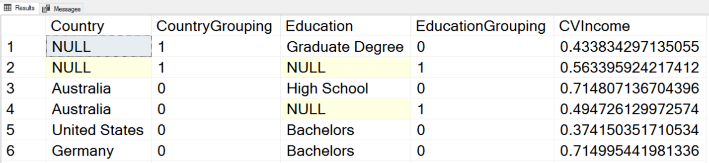
In the first row, you can see that Country is NULL, so this is an aggregate over Education only. In the second row, you can see that both Country and Education are NULL, meaning that this is an aggregate over the whole dataset. I will leave you to interpret the other results by yourself.
Aggregating in R
As you can imagine, there are countless possibilities for aggregating the data in R. In this data science article, I will show you only the options from the base installation, without any additional package. Let me start by reading the data from SQL Server.
|
1 2 3 4 5 6 7 8 9 10 11 |
library(RODBC) con <- odbcConnect("AWDW", uid = "RUser", pwd = "Pa$$w0rd") TM <- as.data.frame(sqlQuery(con, "SELECT g.EnglishCountryRegionName AS Country, c.EnglishEducation AS Education, c.YearlyIncome AS Income FROM dbo.DimCustomer AS c INNER JOIN dbo.DimGeography AS g ON c.GeographyKey = g.GeographyKey;"), stringsAsFactors = TRUE) close(con) |
The first function I want to mention is the summarize() function. It is the simplest way of getting the basic descriptive statistics for a variable, or even for a complete data frame. In the following example, I am analyzing the Income and the Education variables from the TM data frame.
summary(TM$Income)
summary(TM$Education)
Here are the results.
| Min. | 1st Qu. | Median | Mean | 3rd Qu. | Max. |
| 10000 | 30000 | 60000 | 57310 | 70000 | 170000 |
| Bachelors | Graduate Degree | High School | |||
| 5356 | 3189 | 3294 | |||
| Partial College | Partial High School | ||||
| 5064 | 1581 |
You can see that the summary() function returned for a continuous variable the minimal and the maximal values, the values on the first and on the third quartile, and the mean and the median. For a factor, the function returned the absolute frequencies.
There are many other descriptive statistics functions already in base R. The following code shows quite a few of them by analyzing the Income variable.
|
1 2 3 4 5 6 7 8 |
cat(' ','Mean :', mean(TM$Income)) cat('\n','Median:', median(TM$Income)) cat('\n','Min :', min(TM$Income)) cat('\n','Max :', max(TM$Income)) cat('\n','Range :', range(TM$Income)) cat('\n','IQR :', IQR(TM$Income)) cat('\n','Var :', var(TM$Income)) cat('\n','StDev :', sd(TM$Income)) |
The code uses the cat() function which concatenates and prints the parameters. In the result, you can se the mean, the median, the minimal and the maximal value, the range and the inter-quartile range, and the variance and the standard deviation for the Income variable. Here are the results.
| Mean : | 57305.78 |
| Median: | 60000 |
| Min : | 10000 |
| Max : | 170000 |
| Range : | 10000 170000 |
| IQR : | 40000 |
| Var : | 1042375574 |
| StDev : | 32285.84 |
You can use the aggregate() function to aggregate data over groups. Note the three parameters in the following example. The first one is the variable to be aggregated, the second is a list of variables used for grouping, and the third is the aggregate function. In the following example, I am calculating the sum of the income over countries.
|
1 |
aggregate(TM$Income, by = list(TM$Country), FUN = sum) |
As mentioned, the second parameter is a list of variables used to define the grouping. Let me show you an example with two variables in the list by calculating the mean value for the income over countries and education.
|
1 2 3 |
aggregate(TM$Income, by = list(TM$Country, TM$Education), FUN = mean) |
The third parameter is the name of the function. This could also be a custom function. There is no built-in function in the base R installation for calculating the third and the fourth population moments, the skewness and the kurtosis. No problem, it is very easy to write a custom function. The following code shows the function, and then calculates the skewness and the kurtosis for the Income variable over the whole dataset and per country.
|
1 2 3 4 5 6 7 8 9 10 11 |
skewkurt <- function(p) { avg <- mean(p) cnt <- length(p) stdev <- sd(p) skew <- sum((p - avg) ^ 3 / stdev ^ 3) / cnt kurt <- sum((p - avg) ^ 4 / stdev ^ 4) / cnt - 3 return(c(skewness = skew, kurtosis = kurt)) }; skewkurt(TM$Income); # Aggregations in groups with a custom function aggregate(TM$Income, by = list(TM$Country), FUN = skewkurt) |
Here are the results.
| skewness | kurtosis | ||
| 0.8219881 | 0.6451128 | ||
| Group.1 | x.skewness | x.kurtosis | |
| 1 | Australia | -0.05017649 | -0.50240998 |
| 2 | Canada | 0.95311355 | 3.19841011 |
| 3 | France | 1.32590706 | 0.56945630 |
| 4 | Germany | 1.32940136 | 0.35521164 |
| 5 | United Kingdom | 1.34856013 | 0.27294523 |
| 6 | United States | 1.17370389 | 2.08329296 |
If you need to filter the dataset on the aggregated values, you can store the result of the aggregation in a new data frame, and then filter the new data frame, like the following code shows.
|
1 2 3 |
TMAGG <- aggregate(list(Income = TM$Income), by = list(Country = TM$Country), FUN = mean) TMAGG[TMAGG$Income > 60000,] |
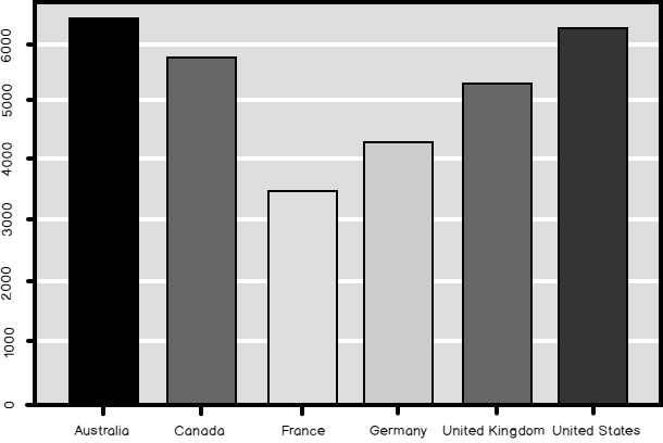
Finally, many of the graphical functions do the grouping and the aggregation by themselves. The barplot() function in the following example plots the bars showing the mean value of the income in each country.
|
1 2 3 |
barplot(TMAGG$Income, legend = TMAGG$Country, col = c('blue', 'yellow', 'red', 'green', 'magenta', 'black')) |
The result is the following graph.
Python Pandas Aggregations
As I explained in my previous article, in Python you get the data frame object when you load the pandas library. This library has also all of the methods you need to aggregate and groups the data and to create simple graphs. The following code imports the necessary libraries and reads the data from SQL Server.
|
1 2 3 4 5 6 7 8 9 10 11 12 13 14 15 |
# Imports needed import numpy as np import pandas as pd import pyodbc import matplotlib.pyplot as plt # Connecting and reading the data con = pyodbc.connect('DSN=AWDW;UID=RUser;PWD=Pa$$w0rd') query = """ SELECT g.EnglishCountryRegionName AS Country, c.EnglishEducation AS Education, c.YearlyIncome AS Income FROM dbo.DimCustomer AS c INNER JOIN dbo.DimGeography AS g ON c.GeographyKey = g.GeographyKey;""" TM = pd.read_sql(query, con) |
The pandas data frame describe() method is quite similar to the R summary() function – provides you a quick overview of a variable. Besides this function, there are many separate descriptive statistics functions implemented as data frame methods as well. The list of these functions includes the functions that calculate the skewness and the kurtosis, as you can see from the following code.
|
1 2 3 4 5 6 |
# Summary TM.describe() # Count and variance TM['Income'].count(), TM['Income'].var() # Skewness and kurtosis TM['Income'].skew(), TM['Income'].kurt() |
Here are the results – descriptive statistics for the Income variable. You should be able to interpret the results by yourself without any problem.
|
1 2 3 4 5 6 7 8 9 10 11 12 13 14 |
>>> # Summary Income count 18484.000000 mean 57305.777970 std 32285.841703 min 10000.000000 25% 30000.000000 50% 60000.000000 75% 70000.000000 max 170000.000000 >>> # Count and variance (18484, 1042375574.4691552) >>> # Skewness and kurtosis (0.82212157713655321, 0.64600652578292239) |
The pandas data frame groupby() method allows you to calculate the aggregates over groups. You can see in the following example calculation of counts, medians, and descriptive statistics of the Income variable over countries.
|
1 2 3 |
TM.groupby('Country')['Income'].count() TM.groupby('Country')['Income'].median() TM.groupby('Country')['Income'].describe() |
For the sake of brevity, I am showing only the counts here.
| Country | |
| Australia | 3591 |
| Canada | 1571 |
| France | 1810 |
| Germany | 1780 |
| United Kingdom | 1913 |
| United States | 7819 |
If you need to filter the dataset based on the aggregated values, you can do it in the same way as in R. You store the results in a new data frame, and then filter the new data frame, like the following code shows.
|
1 2 |
TMAGG = pd.DataFrame(TM.groupby('Country')['Income'].median()) TMAGG.loc[TMAGG.Income > 50000] |
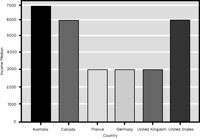
Like the R graphing functions also the pandas data frame plot() function groups the data for you. The following code generates a bar chart with the medain income per country.
|
1 2 3 4 5 6 7 |
ax = TMAGG.plot(kind = 'bar', colors = ('b', 'y', 'r', 'g', 'm', 'k'), fontsize = 14, legend = False, use_index = True, rot = 1) ax.set_xlabel('Country', fontsize = 16) ax.set_ylabel('Income Median', fontsize = 16) plt.show() |
And here is the bar chart as the final result of the code in this data science article. Compare the median and the mean (shown in the graph created with the R code) of the Income in different countries.
Conclusion
I am not done with grouping and aggregating in this series of Data science articles yet. In the following article, I plan to show you some advanced examples of GROUPING SETS clause in T-SQL. I will show you how to use some efficient grouping and aggregating methods in R by using external packages. I will do an additional deep dive in pandas data frame options for grouping and aggregating data.
Table of contents
References
- AggregatFunctions (Transact-SQL) in Microsoft Docs
- SELECT – GROUP BY (Transact-SQL) in Microsoft Docs
- GROUPING (Transact-SQL) in Microsoft Docs
- R summary function
- Concatenate and print – cat R function
- Compute summary statistics of data subsets – aggregate in R
- Skewness and kurtosis in the NIST/SEMATECH e-Handbook of Statistical Methods
- The pandas data frame describe() function
- The pandas data frame groupby() function

View all posts by Dejan Sarka
- Data Science in SQL Server: Unpivoting Data - October 29, 2018
- Data science in SQL Server: Data analysis and transformation – Using SQL pivot and transpose - October 11, 2018
- Data science in SQL Server: Data analysis and transformation – grouping and aggregating data II - September 28, 2018