
You might find the T-SQL GROUPING SETS I described in my previous data science article a bit complex. However, I am not done with it yet. I will show additional possibilities in this article. But before you give up on reading the article, let me tell you that I will also show a way how to make R code simpler with help of the dplyr package. Finally, I will also show some a bit more advanced techniques of aggregations in Python pandas data frame.
T-SQL Grouping Sets Subclauses
Let me start immediately with the first GROUPINS SETS query. The following query calculates the sum of the income over countries and states, over whole countries, and finally over the whole rowset. Aggregates over whole countries are sums of aggregates over countries and states; the SQL aggregate over the whole rowset is a sum of aggregates over countries. SQL Server can calculate all of the aggregations needed with a single scan through the data.
|
1 2 3 4 5 6 7 8 9 10 11 12 13 |
USE AdventureWorksDW2016; SELECT g.EnglishCountryRegionName AS Country, g.StateProvinceName AS StateProvince, SUM(c.YearlyIncome) AS SumIncome FROM dbo.DimCustomer AS c INNER JOIN dbo.DimGeography AS g ON c.GeographyKey = g.GeographyKey GROUP BY GROUPING SETS ( (g.EnglishCountryRegionName, g.StateProvinceName), (g.EnglishCountryRegionName), () ); |
The previous query can be shortened with the ROLLUP clause. Look at the following query.
|
1 2 3 4 5 6 7 8 |
SELECT g.EnglishCountryRegionName AS Country, g.StateProvinceName AS StateProvince, SUM(c.YearlyIncome) AS SumIncome FROM dbo.DimCustomer AS c INNER JOIN dbo.DimGeography AS g ON c.GeographyKey = g.GeographyKey GROUP BY ROLLUP (g.EnglishCountryRegionName, g.StateProvinceName); |
The ROLLUP clause rolls up the subtotal to the subtotals on the higher levels and to the grand total. Looking at the clause, it creates hyper-aggregates on the columns in the clause from right to left, in each pass decreasing the number of columns over which the aggregations are calculated. The ROLLUP clause calculates only those aggregates that can be calculated within a single pass through the data.
There is another shortcut command for the GROUPING SETS – the CUBE command. This command creates groups for all possible combinations of columns. Look at the following query.
|
1 2 3 4 5 6 7 8 |
SELECT c.Gender, c.MaritalStatus, SUM(c.YearlyIncome) AS SumIncome FROM dbo.DimCustomer AS c INNER JOIN dbo.DimGeography AS g ON c.GeographyKey = g.GeographyKey GROUP BY CUBE (c.Gender, c.MaritalStatus); |
Here is the result.
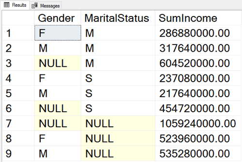
You can see the aggregates over Gender and MaritaStatus, hyper-aggregates over Gender only and over MaritalStatus only, and the hyper-aggregate over the complete input rowset.
I can write the previous query in another way. Note that the GROUPING SETS clause says “sets” in plural. So far, I defined only one set in the clause. Now take a loot at the following query.
|
1 2 3 4 5 6 7 8 9 10 11 12 |
SELECT c.Gender, c.MaritalStatus, SUM(c.YearlyIncome) AS SumIncome FROM dbo.DimCustomer AS c INNER JOIN dbo.DimGeography AS g ON c.GeographyKey = g.GeographyKey GROUP BY GROUPING SETS ( (c.Gender), () ), ROLLUP(c.MaritalStatus); |
The query has two sets defined: grouping over Gender and over the whole rowset, and then, in the ROLLUP clause, grouping over MaritalStatus and over the whole rowset. The actual grouping is over the cartesian product of all sets in the GROUPING SETS clause. Therefore, the previous query calculates the aggregates over Gender and MaritaStatus, the hyper-aggregates over Gender only and over MaritalStatus only, and the hyper-aggregate over the complete input rowset. If you add more columns in each set, the number of grouping combinations raises very quickly, and it becomes very hard to decipher what the query actually does. Therefore, I would recommend you to use this advanced way of defining the GROUPING SETS clause very carefully.
There is another problem with the hyper-aggregates. In the rows with the hyper-aggregates, there are some columns showing NULL. This is correct, because when you calculate in the previous query the hyper-aggregate over the MaritalStatus column, then the value of the Gender column is unknown, and vice-versa. For the aggregate over the whole rowset, the values of both columns are unknown. However, there could be another reason to get NULLs in those two columns. There might be already NULLs in the source dataset. Now you need to have a way to distinguish the NULLs in the result that are the NULLs aggregated over the NULLs in the source data in a single group and the NULLs that come in the result because of the hyper-aggregates. Here the GROUPING() AND GROUPING_ID functions become handy. Look at the following query.
|
1 2 3 4 5 6 7 8 9 10 11 12 |
SELECT GROUPING(c.Gender) AS GroupingG, GROUPING(c.MaritalStatus) AS GroupingM, GROUPING_ID(c.Gender, c.MaritalStatus) AS GroupingId, c.Gender, c.MaritalStatus, SUM(c.YearlyIncome) AS SumIncome FROM dbo.DimCustomer AS c INNER JOIN dbo.DimGeography AS g ON c.GeographyKey = g.GeographyKey GROUP BY CUBE (c.Gender, c.MaritalStatus); |
Here is the result.
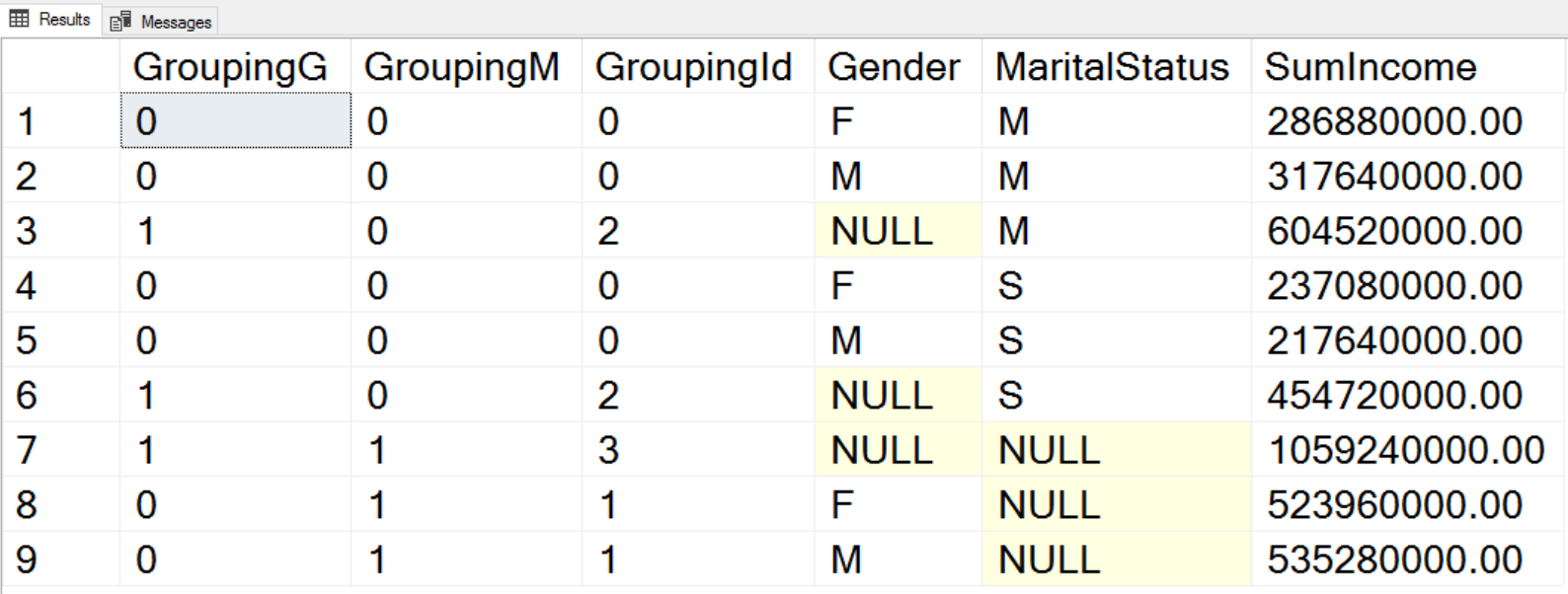
The GROUPING() function accepts a single column as an argument and returns 1 if the NULL in the column is because it is a hyper-aggregate when the column value is not applicable, and 0 otherwise. For example, in the third row of the output, you can see that this is the aggregate over the MaritalStatus only, where Gender makes no sense, and the GROUPING(Gender) returns 1. If you read my previous article, you probably already know this function. I introduced it there, together with the problem is solves.
The GROUPING_ID() function is another solution for the same problem. It accepts both columns as the argument and returns an integer bitmap for the hyper-aggregates fo these two columns. Look at the last row in the output. The GROUPING() function returs in the first two columns values 0 and 1. Let’s write them thether as a bitmap and get 01. Now let’s calculate the integer of the bitmap: 1×20 + 0x21 = 1. Ths means that the MaritalStatus NULL is there because this is a hyper-aggregate over the Gender only. Now chect the sevents row. The bitmap calulation to integer is: 1×20 + 0x21 = 3. So this is the hyper-aggregate where none of the two inpuc columns are applicable, the hyper-aggregate over the whole rowset.
Introducing the dplyr Package
After the complex GROUPING SETS clause, I guess you will appreciate the simplicity of the following R code. Let me quickly read the data from SQL Server in R.
|
1 2 3 4 5 6 7 8 9 10 11 12 13 14 15 16 17 |
library(RODBC) con <- odbcConnect("AWDW", uid = "RUser", pwd = "Pa$$w0rd") TM <- as.data.frame(sqlQuery(con, "SELECT c.CustomerKey, g.EnglishCountryRegionName AS Country, g.StateProvinceName AS StateProvince, c.EnglishEducation AS Education, c.NumberCarsOwned AS TotalCars, c.MaritalStatus, c.TotalChildren, c.NumberChildrenAtHome, c.YearlyIncome AS Income FROM dbo.DimCustomer AS c INNER JOIN dbo.DimGeography AS g ON c.GeographyKey = g.GeographyKey;"), stringsAsFactors = TRUE) close(con) |
I am going to install the dplyr package. This is a very popular package for data manipulation in r. It brings simple and concise syntax. Let me install it and load it.
|
1 2 |
install.packages("dplyr") library(dplyr) |
The first function to introduce from the dplyr package is the glimpse() function. If returns a brief overview of the variables in the data frame. Here is the call of that function.
|
1 |
glimpse(TM) |
Bellow is a narrowed result.
|
1 2 3 4 5 6 7 8 9 |
$ CustomerKey <int> 11000, 11001, 11002, 11003, 11004, 11005, $ Country <fctr> Australia, Australia, Australia, Australi $ StateProvince <fctr> Queensland, Victoria, Tasmania, New South $ Education <fctr> Bachelors, Bachelors, Bachelors, Bachelor $ TotalCars <int> 0, 1, 1, 1, 4, 1, 1, 2, 3, 1, 1, 4, 2, 3, $ MaritalStatus <fctr> M, S, M, S, S, S, S, M, S, S, S, M, M, M, $ TotalChildren <int> 2, 3, 3, 0, 5, 0, 0, 3, 4, 0, 0, 4, 2, 2, $ NumberChildrenAtHome <int> 0, 3, 3, 0, 5, 0, 0, 3, 4, 0, 0, 4, 0, 0, $ Income <dbl> 9e+04, 6e+04, 6e+04, 7e+04, 8e+04, 7e+04, |
The dplyr package brings functions that allow you to manipulate the data with the syntax that briefly resembles the T-SQL SELECT statement. The select() function allows you to define the projection on the dataset, to select specific columns only. The following code uses the head() basic R function to show the first six rows. Then the second line uses the dplyr select() function to select only the columns from CustomerKey to TotalCars. The third line selects only columns with the word “Children” in the name. The fourth line selects only columns with the name that starts with letter “T”.
|
1 2 3 4 |
head(TM) head(select(TM, CustomerKey:TotalCars)) head(select(TM, contains("Children"))) head(select(TM, starts_with("T"))) |
For the sake of brevity, I am showing the results of the last line only.
|
1 2 3 4 5 6 7 |
TotalCars TotalChildren 1 0 2 2 1 3 3 1 3 4 1 0 5 4 5 6 1 0 |
The filter() function allows you to filter the data similarly like the T-SQL WHERE clause. Look at the following two examples.
|
1 2 3 4 5 |
# Filter filter(TM, CustomerKey < 11005) # With projection select(filter(TM, CustomerKey < 11005), TotalCars, MaritalStatus) |
Again, I am showing the results of the last command only.
|
1 2 3 4 5 6 |
TotalCars MaritalStatus 1 0 M 2 1 S 3 1 M 4 1 S 5 4 S |
The dplyr package also defines the very useful pipe operator, written as %>%. It allows you to chain the commands. The output of one command is the input for the following function. The following code is equivalent to the previous one, just that it uses the pipe operator.
|
1 2 3 |
TM %>% filter(CustomerKey < 11005) %>% select(TotalCars, MaritalStatus) |
The distinct() function work similarly like the T-SQL DISTINCT clause. The following code uses it.
|
1 2 3 4 |
TM %>% filter(CustomerKey < 11005) %>% select(TotalCars, MaritalStatus) %>% distinct |
Here is the result.
|
1 2 3 4 5 |
TotalCars MaritalStatus 1 0 M 2 1 S 3 1 M 4 4 S |
You can also use the dplyr package for sampling the rows. The sample_n() function allows you to select n random rows with replacement and without replacement, as the following code shows.
# Sampling with replacement
|
1 2 3 4 5 6 7 8 9 10 |
# Sampling with replacement TM %>% filter(CustomerKey < 11005) %>% select(CustomerKey, TotalCars, MaritalStatus) %>% sample_n(3, replace = TRUE) # Sampling without replacement TM %>% filter(CustomerKey < 11005) %>% select(CustomerKey, TotalCars, MaritalStatus) %>% sample_n(3, replace = FALSE) |
Here is the result.
|
1 2 3 4 5 6 7 8 |
CustomerKey TotalCars MaritalStatus 3 11002 1 M 3.1 11002 1 M 1 11000 0 M CustomerKey TotalCars MaritalStatus 3 11002 1 M 1 11000 0 M 2 11001 1 S |
|
1 2 3 4 5 6 |
CustomerKey TotalCars MaritalStatus 3 11002 1 M 1 11000 0 M 2 11001 1 S |
Note that when sampling with replacement, the same row can come in the sample multiple times. Also, note that the sampling is random; therefore, the next time you execute this code you will probably get different results.
The arrange() function allows you to reorder the data frame, similarly to the T-SQL OREDER BY clause. Again, for the sake of brevity, I am not showing the results for the following code.
|
1 2 |
head(arrange(select(TM, CustomerKey:StateProvince), desc(Country), StateProvince)) |
The mutate() function allows you to add calculated columns to the data frame, like the following code shows.
|
1 2 3 4 |
TM %>% filter(CustomerKey < 11005) %>% select(CustomerKey, TotalChildren, NumberChildrenAtHome) %>% mutate(NumberChildrenAway = TotalChildren - NumberChildrenAtHome) |
Here is the result.
|
1 2 3 4 5 6 |
CustomerKey TotalChildren NumberChildrenAtHome NumberChildrenAway 1 11000 2 0 2 2 11001 3 3 0 3 11002 3 3 0 4 11003 0 0 0 5 11004 5 5 0 |
Finally, let’s do the aggregations, like the title of this article promises. You can use the summarise() function for that task. For example, the following line of code calculates the average value for the Income variable.
|
1 |
summarise(TM, avgIncome = mean(Income)) |
You can also calculates aggregates in groups with the group_by() function.
|
1 |
summarise(group_by(TM, Country), avgIncome = mean(Income)) |
Here is the result.
|
1 2 3 4 5 6 7 8 |
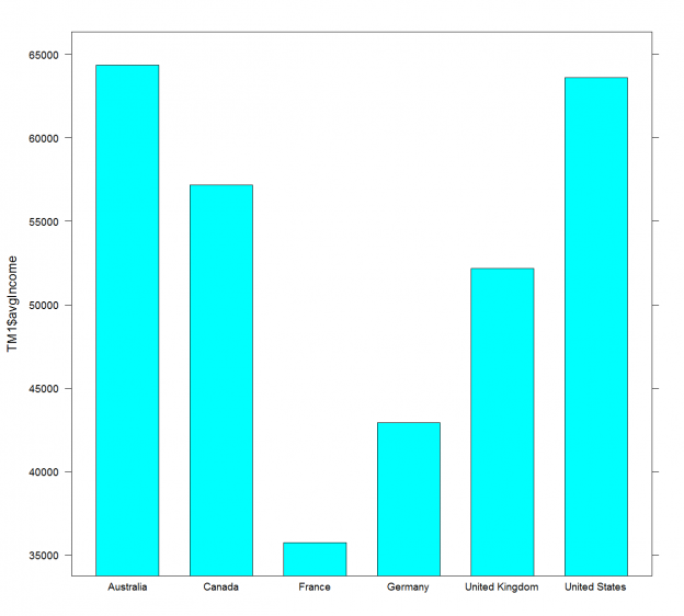
Country avgIncome <fctr> <dbl> 1 Australia 64338.62 2 Canada 57167.41 3 France 35762.43 4 Germany 42943.82 5 United Kingdom 52169.37 6 United States 63616.83 |
The top_n() function works similarly to the TOP T-SQL clause. Look at the following code.
|
1 2 3 4 5 6 |
summarise(group_by(TM, Country), avgIncome = mean(Income)) %>% top_n(3, avgIncome) %>% arrange(desc(avgIncome)) summarise(group_by(TM, Country), avgIncome = mean(Income)) %>% top_n(-2, avgIncome) %>% arrange(avgIncome) |
I am calling the top_n() function twice, to calculate the top 3 countries by average income and the bottom two. Note that the order of the calculation is defined by the sign of the number of rows parameter. In the first call, 3 means the top 3 descending, and in the second call, 2 means top two in ascending order. Here is the result of the previous code.
|
1 2 3 4 5 |
Country avgIncome <fctr> <dbl> 1 Australia 64338.62 2 United States 63616.83 3 Canada 57167.41 |
|
1 2 3 4 |
Country avgIncome <fctr> <dbl> 1 France 35762.43 2 Germany 42943.82 |
Finally, you can store the results of the dplyr functions in a normal data frame. The following code creates a new data frame and then shows the data graphically.
|
1 2 3 |
TM1 = summarise(group_by(TM, Country), avgIncome = mean(Income)) barchart(TM1$avgIncome ~ TM1$Country) |
The result is the following graph.
Advanced Python Pandas Aggregations
Time to switch to Python. Again, I need to start with importing the necessary libraries and reading the data.
|
1 2 3 4 5 6 7 8 9 10 11 12 13 14 |
import numpy as np import pandas as pd import pyodbc import matplotlib.pyplot as plt con = pyodbc.connect('DSN=AWDW;UID=RUser;PWD=Pa$$w0rd') query = """ SELECT g.EnglishCountryRegionName AS Country, c.EnglishEducation AS Education, c.YearlyIncome AS Income, c.NumberCarsOwned AS Cars FROM dbo.DimCustomer AS c INNER JOIN dbo.DimGeography AS g ON c.GeographyKey = g.GeographyKey;""" TM = pd.read_sql(query, con) |
From the previous article, you probably remember the describe() function. The following code uses it to calculate the descriptive statistics for the Income variable over countries.
|
1 |
TM.groupby('Country')['Income'].describe() |
Here is an abbreviated result.
|
1 2 3 4 5 6 7 8 9 10 11 12 |
Country Australia count 3591.000000 mean 64338.624339 std 31829.998608 min 10000.000000 25% 40000.000000 50% 70000.000000 75% 80000.000000 max 170000.000000 Canada count 1571.000000 mean 57167.409293 std 20251.523043 |
You can use the unstack() function to get a tabular result:
|
1 |
TM.groupby('Country')['Income'].describe().unstack() |
Here is the narrowed tabular result.
|
1 2 3 4 5 6 7 8 |
count mean std Country Australia 3591.0 64338.624339 31829.998608 Canada 1571.0 57167.409293 20251.523043 France 1810.0 35762.430939 27277.395389 Germany 1780.0 42943.820225 35493.583662 United Kingdom 1913.0 52169.367486 48431.988315 United States 7819.0 63616.830797 25706.482289 |
You can use the SQL aggregate() function to calculate multiple aggregates on multiple columns at the same time. The agg() is a synonym for the SQL aggregate(). Look at the following example.
|
1 2 3 4 |
TM.groupby('Country').aggregate({'Income': 'std', 'Cars':'mean'}) TM.groupby('Country').agg({'Income': ['max', 'mean'], 'Cars':['sum', 'count']}) |
The first call calculates a single SQL aggregate for two variables. The second call calculates two aggregates for two variables. Here is the result of the second call.
|
1 2 3 4 5 6 7 8 9 |
Cars Income sum count max mean Country Australia 6863 3591 170000.0 64338.624339 Canada 2300 1571 170000.0 57167.409293 France 2259 1810 110000.0 35762.430939 Germany 2162 1780 130000.0 42943.820225 United Kingdom 2325 1913 170000.0 52169.367486 United States 11867 7819 170000.0 63616.830797 |
You might dislike the form of the previous result because the names of the columns are written in two different rows. You might want to flatten the names to a single word for a column. You can use the numpy ravel() function to latten the array of the column names and then concatenate them to a single name, like the following code shows.
|
1 2 3 4 5 6 7 8 9 10 11 12 |
# Renaming the columns IncCars = TM.groupby('Country').aggregate( {'Income': ['max', 'mean'], 'Cars':['sum', 'count']}) # IncCars # Ravel function # IncCars.columns # IncCars.columns.ravel() # Renaming IncCars.columns = ["_".join(x) for x in IncCars.columns.ravel()] # IncCars.columns IncCars |
You can also try to execute the commented code to get the understanding how the ravel() function works step by step. Anyway, here is the final result.
|
1 2 3 4 5 6 7 8 |
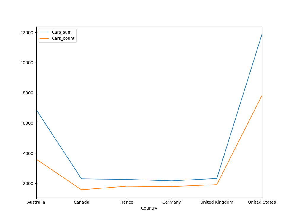
Cars_sum Cars_count Income_max Income_mean Country Australia 6863 3591 170000.0 64338.624339 Canada 2300 1571 170000.0 57167.409293 France 2259 1810 110000.0 35762.430939 Germany 2162 1780 130000.0 42943.820225 United Kingdom 2325 1913 170000.0 52169.367486 United States 11867 7819 170000.0 63616.830797 |
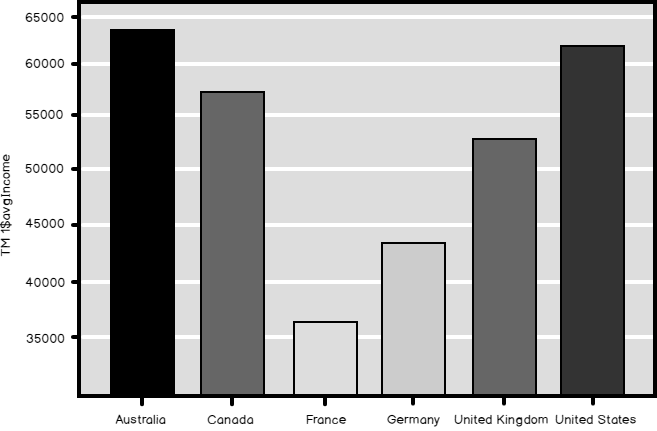
For a nice end, let me show you the results also graphically.
|
1 2 |
IncCars[['Cars_sum','Cars_count']].plot() plt.show() |
And here is the graph.
Conclusion
I will finish with aggregations in this data science series for now. However, I am not done with data preparation yet. You will learn about other problems and solutions in the forthcoming data science articles.
Table of contents

View all posts by Dejan Sarka
- Data Science in SQL Server: Unpivoting Data - October 29, 2018
- Data science in SQL Server: Data analysis and transformation – Using SQL pivot and transpose - October 11, 2018
- Data science in SQL Server: Data analysis and transformation – grouping and aggregating data II - September 28, 2018