
In this article, in the data science: data analysis and transformation series, we’ll be talking about information entropy.
In the conclusion of my last article, Data science, data understanding and preparation – binning a continuous variable, I wrote something about preserving the information when you bin a continuous variable to bins with an equal number of cases. I am explaining this sentence in this article you are currently reading. I will show you how to calculate the information stored in a discrete variable by explaining the measure for the information, namely the information entropy.
Information entropy was defined by Claude E. Shannon in his information theory. Shannon’s goal was to quantify the amount of information in a variable. Nowadays the information theory as a special branch of applied mathematics is used in many places, such as computer science, electrical engineering, and more.
Introducing information entropy
Information is actually a surprise. If you are surprised when you hear or read something, this means that you didn’t know that, that you actually learned something new, and this something new is a piece of information. So how does this connect to a variable in your dataset?
Intuitively, you can imagine that the information of a variable is connected with its variability. If a variable is a constant, where all cases occupy the same single state, you cannot be surprised with a value of any single case. Imagine that you have a group of attendees in a classroom. You know a bit about their education. Let’s start with an example where you split the attendees into two groups by the education: low and high. In one class, 95% of attendees have high and 5% low education. You ask a random attendee about her or his actual education level. You would expect that it would be high. You would be surprised only in 5% of cases, learning that for that particular attendee is actually low. Now imagine that you have a 50% – 50% case. The knowledge about this distribution does not help you much – whatever state you would expect; you would be surprised half of the times.
Now imagine that you have previous knowledge about the attendees’ education classified into three distinct classes: low, medium, and high. With a distribution 33% – 33% – 33%, you would be surprised about some person’s education in two thirds of the cases. With any other distribution, for example 25% – 50% – 25%, you would be surprised fewer times. For this specific case, you would expect medium level, and half of the times you would learn that the level of the person you are talking with is not medium, being either low or high.
From last two paragraphs, you can see that more possible states mean higher maximal possible surprise or maximal possible information. By binning, you are lowering the number of possible states. If you bin to classes with equal height, the loss of the information is minimal, preserving it as much as possible, as I wrote in my previous article.
Of course, the question is how to measure this information. You can try to measure the spread of the variable. For example, for ordinal variables stored as integers, you could pretend that the variables are continuous, and you could use standard deviation as a measure. In order to compare the spread of two different variables, you could use the relative variability, of the coefficient of variation, defined as standard deviation divided by the mean:

Let me start by preparing the demo data for this article with T-SQL. Note that I created a calculated variable GenMar by simply concatenating the Gender and the MaritalStatus variables into on that will have four distinct stated (FM, FS, MM, MS).
|
1 2 3 4 5 6 7 8 9 10 11 |
USE AdventureWorksDW2016; GO -- Preparing demo table DROP TABLE IF EXISTS dbo.TM; GO SELECT CustomerKey, NumberCarsOwned, BikeBuyer, Gender + MaritalStatus AS GenMar INTO dbo.TM FROM dbo.vTargetMail; GO |
Now I will switch to R. Here is the code that reads the data from the table I just created.
|
1 2 3 4 5 6 7 8 9 10 |
# Load RODBC library (install only if needed) # install.packages("RODBC") library(RODBC) # Connecting and reading the data con <- odbcConnect("AWDW", uid = "RUser", pwd = "Pa$$w0rd") TM <- as.data.frame(sqlQuery(con, "SELECT CustomerKey, NumberCarsOwned, BikeBuyer, GenMar FROM dbo.TM;"), stringsAsFactors = TRUE) close(con) |
In this article, I will use the RevoScaleR package for drawing the histogram, and DescTools package for calculating the information entropy, so you need to load them, and potentially also install the DescTools package (you should already have the RevoScaleR package if you use the Microsoft R engine).
|
1 2 3 4 5 |
# Histogram from RevoScaleR # Information entropy (install only if needed) from DescTools # install.packages("DescTools"); library("RevoScaleR") library("DescTools") |
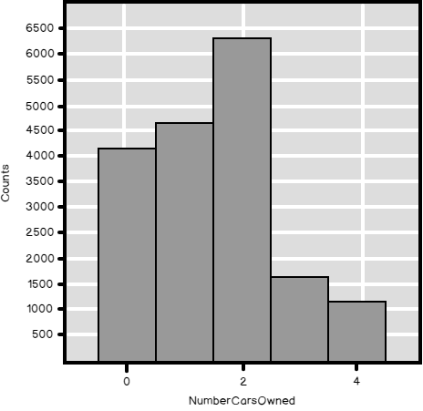
The following R code calculates the frequencies, creates a histogram, and calculates the mean, standard deviation, and coefficient of variation for the NumberCarsOwned variable. Note that I use the paste() function to concatenate the strings with the calculated values.
|
1 2 3 4 5 6 7 8 |
# Frequencies and histogram table(TM$NumberCarsOwned) rxHistogram(formula = ~NumberCarsOwned, data = TM) # Mean, StDev, CV paste('mean:', mean(TM$NumberCarsOwned)) paste('sd :', sd(TM$NumberCarsOwned)) paste('CV :', sd(TM$NumberCarsOwned) / mean(TM$NumberCarsOwned)) |
Here is the histogram for this variable.

And here are the numerical results.
| 0 | 1 | 2 | 3 | 4 |
| 4238 | 4883 | 6457 | 1645 | 1261 |
| [1] “mean: 1.50270504219866” |
| [1] “sd : 1.13839374115481” |
| [1] “CV : 0.757563000846255” |
Let me do the same calculations for the BikeBuyer variable.
|
1 2 3 4 |
table(TM$BikeBuyer) paste('mean:', mean(TM$BikeBuyer)) paste('sd :', sd(TM$BikeBuyer)) paste('CV :', sd(TM$BikeBuyer) / mean(TM$BikeBuyer)) |
Here are the results.
| 0 | 1 |
| 9352 | 9132 |
| [1] “mean: 0.494048907162952” |
| [1] “sd : 0.499978108041433” |
| [1] “CV : 1.01200124277681” |
You can see that although the standard deviation for the BikeBuyer is lower than for the NumberCarsOwned, the relative variability is higher.
Now, what about the categorical, or nominal variables? Of course, you cannot use the calculations that are intended for the continuous variables. Time to calculate the information entropy.
Defining information entropy
Shannon defined the information of a particular state as a probability multiplied by the logarithm with base two of the probability:
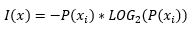
The probability can take a value in an interval between 0 and 1. The logarithm function returns negative values for the interval between zero and one. This is why the negative sign, or the multiplication by -1, is added.
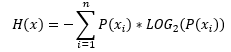
The information entropy of a variable, or the actual amount of information stored in this variable, is simply a sum of information of all particular states:
What is the maximal possible entropy for a specific number of states, let’s say three? Let’s do the calculation.

From logarithm formulas, we know that we can express
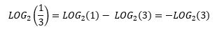
Therefore, we can develop the equation for the maximal possible information entropy:
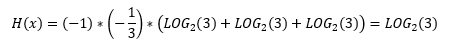
You can see that the maximal possible information entropy of a variable with n states is logarithm base two of this number n.
Calculating the entropy in T-SQL
Let me start with a calculation of the maximal possible information entropy for a different number of states.
|
1 2 3 4 |
SELECT LOG(2,2) AS TwoStatesMax, LOG(3,2) AS ThreeStatesMax, LOG(4,2) AS FourStatesMax, LOG(5,2) AS FiveStatesMax; |
Here are the results.

The following code calculates the frequencies of the GenMar variable, the information entropy for each state, and then the total entropy, compared to the maximal possible information entropy of a four-state variable.
|
1 2 3 4 5 6 7 8 9 10 11 12 13 14 15 16 17 18 19 20 21 |
-- Entropy of the GenMar WITH ProbabilityCTE AS ( SELECT GenMar, COUNT(GenMar) AS StateFreq FROM dbo.TM GROUP BY GenMar ), StateEntropyCTE AS ( SELECT GenMar, 1.0*StateFreq / SUM(StateFreq) OVER () AS StateProbability FROM ProbabilityCTE ) SELECT 'GenMar' AS Variable, (-1)*SUM(StateProbability * LOG(StateProbability,2)) AS TotalEntropy, LOG(COUNT(*),2) AS MaxPossibleEntropy, 100 * ((-1)*SUM(StateProbability * LOG(StateProbability,2))) / (LOG(COUNT(*),2)) AS PctOfMaxPossibleEntropy FROM StateEntropyCTE; GO |
From the results, you can see that this variable has a high relative entropy.

Calculating the information entropy in Python
For a start, let’s import all of the libraries needed and read the data.
|
1 2 3 4 5 6 7 8 9 10 11 12 |
# Imports needed import numpy as np import pandas as pd import pyodbc import matplotlib.pyplot as plt import seaborn as sns import scipy as sc # Connecting and reading the data con = pyodbc.connect('DSN=AWDW;UID=RUser;PWD=Pa$$w0rd') query = """SELECT CustomerKey, NumberCarsOwned, BikeBuyer, GenMar FROM dbo.TM;""" TM = pd.read_sql(query, con) |
For the calculation of the information entropy, you can use the scipy.stat.entropy() function. This function need the probabilities as the input. Therefore, I defined my own function that calculates the entropy with a single argument – the name of the variable, and then in the body I calculate the state probabilities and the entropy of the variable with the scipy.stats.entropy() function. Then I calculate the information entropy of the discrete variables I have in my dataset.
|
1 2 3 4 5 6 7 8 9 |
# Function that calculates the entropy def f_entropy(indata): indataprob = indata.value_counts() / len(indata) entropy=sc.stats.entropy(indataprob, base = 2) return entropy # Use the function on variables f_entropy(TM.NumberCarsOwned), np.log2(5), f_entropy(TM.NumberCarsOwned) / np.log2(5) f_entropy(TM.BikeBuyer), np.log2(2), f_entropy(TM.BikeBuyer) / np.log2(2) f_entropy(TM.GenMar), np.log2(4), f_entropy(TM.GenMar) / np.log2(4) |
Here are the results.
| (2.0994297487400737, 2.3219280948873622, 0.9041751781042634) |
| (0.99989781003755662, 1.0, 0.99989781003755662) |
| (1.9935184517263986, 2.0, 0.99675922586319932) |
Calculating information entropy in R
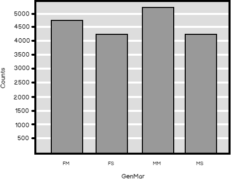
Finally, let’s do the calculation of the information entropy also in R. But before that, let me show you the distribution and the histogram for the GenMar calculated variable.
|
1 2 3 4 |
# GenMar table(TM$GenMar) rxHistogram(formula = ~GenMar, data = TM) |
Here are the numerical and graphical results.
| FM | FS | MM | MS |
| 4745 | 4388 | 5266 | 4085 |
In R, I will use the DescTools Entropy() function. This function expects the absolute frequencies as the input. Here you can see the code.
|
1 2 3 4 5 6 7 |
# Entropy NCOT = table(TM$NumberCarsOwned) print(c(Entropy(NCOT), log2(5), Entropy(NCOT) / log2(5))) BBT = table(TM$BikeBuyer) print(c(Entropy(BBT), log2(2), Entropy(BBT) / log2(2))) GenMarT = table(TM$GenMar) print(c(Entropy(GenMarT), log2(4), Entropy(GenMarT) / log2(4))) |
And here are the last results in this article.
| [1] 2.0994297 2.3219281 0.9041752 |
| [1] 0.9998978 1.0000000 0.9998978 |
| [1] 1.9935185 2.0000000 0.9967592 |
Conclusion
This concludes my article on information entropy. After exhausting articles on working with discrete variables, it looks like it would be time for switching to continuous ones. But before that, I want to explain something else. In some of my previous articles, I tacitly added calculated variables to a dataset. Therefore, I want to introduce some of the operations on the whole datasets.
Table of contents
References
- R paste()function documentation
- Python scipy.stat.entropy()function documentation
- R DescTools Entropy()function documentation

View all posts by Dejan Sarka
- Data Science in SQL Server: Unpivoting Data - October 29, 2018
- Data science in SQL Server: Data analysis and transformation – Using SQL pivot and transpose - October 11, 2018
- Data science in SQL Server: Data analysis and transformation – grouping and aggregating data II - September 28, 2018