
Some time ago, on the 24HOP Russia I was talking about the Query Processor internals and joins. Despite I had three hours, I felt the lack of time, and something left behind, because it is a huge topic, if you try to cover it in different aspects in details. With the few next articles, I’ll try to describe some interesting parts of my talk in more details. I will start with Hash Join execution internals.
The Hash Match algorithm is one of the three available algorithms for joining two tables together. However, it is not only about joining. You may observe a complete list of the logical operations that Hash Match supports in the documentation:
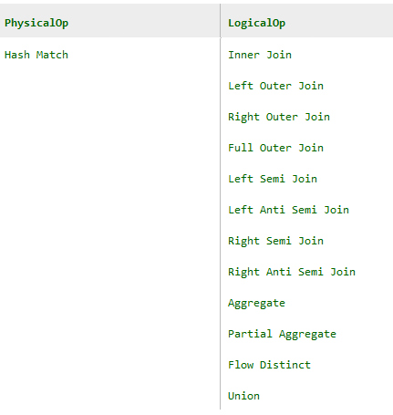
There are quite interesting logical operators implemented by Hash Match, like Partial Aggregate, or even more exotic Flow Distinct. Still, all that is very interesting, the focus of this post is on the Hash Match execution internals in the inner join row mode for regular tables (not in-memory tables).
In memory Algorithm
The simplified process as a whole might be illustrated as follows.
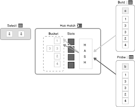
Hash Match in the join mode consumes two inputs, as we are joining two tables. The main idea is to build the hash table using the first “build” input, and then apply the same approach hash the second “probe” input to see if there will be matches of hashed values.
Query Processor (QP) is doing many efforts while building the plan to choose the correct join order. From the Hash Match prospective, it means that QP should choose what table is on the Build side and what is on the Probe side. The Build size should be smaller as it will be stored in memory when building a hash table.
Building a hash table begins with hashing join key values of the build table and placing them to one or another bucket depending on the hash value. Then QP starts processing the probe side, it applies the same hash function to the probe values, determining the bucket and compares the values inside of the bucket. If there is a match – the row is returned.
That would be the whole story if we had infinite memory, but in the real world, it is not true. More to the point, SQL Server allocates memory to the query before the execution starts and does not change it during the execution. That means that if the allocated memory amount is much less than the data size came during the execution, a Hash Match should be able to partition the joining data, and process it in portions that fit allocated memory, while the rest of the data is spilled to the disk waiting to be processed. Here is where the dancing begins.
General Algorithm
A couple of pictures to illustrate the algorithm. The first one depicts the structures.

Build – first input, used to build a hash table.
Probe – second input used to check on a hash table.
Hash Table – an array of slots.
Hash Bucket – a linked list anchored to a slot.
Partition – a group of buckets.
Hash – the hash function applied to the joining value.
Worktable – table located in memory and used to save build input rows.
Workfile – space in tempdb used to store the data that do not fit in the Worktable.
Bitmap – internal hash bit-vector used to optimize spilling/reading to/from the Workfile (in case of dual input).
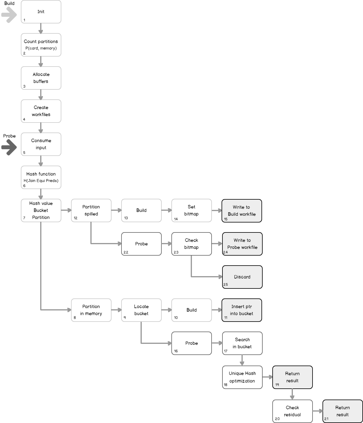
The second one is the logical algorithm. Let’s go through it step by step.
- QP begins by initializing some base objects and structures for further operations.
- Then based on the input (build) cardinality and memory size QP calculates in how many logical groups, i.e. partitions it should divide the input build set.
- QP allocates memory in the buffer pool for each of the partitions – that would be a Worktable.
- QP initializes two empty files per partition (one for the build input, and one for the probe input) in tempdb, that would be the Workfile for spilling the data.
- The processing begins with starting consuming the build input.
- The hash function is applied to the joining value, only equality predicate values considered to be a hash key for the hash function, inequality will be checked later as residual predicates.
- Hashing result is determined, so the slot, bucket and partition is also determined.
- Check if the partition to which the value belongs to is in memory.
- If it is, locate bucket
- Check, if it is a build phase
- If it is a build phase, than QP should build a hash table, so insert the row into the hash table, however, the whole row is not inserted into the hash table. The hash value and the pointer to the row is inserted, the row goes to the Worktable.
- The next build value is coming and goes through steps 5-7, imagine that partition determined for this value is spilled.
- Check, is a build phase.
- If it is, then set the bitmap filter for optimizing the probe checks in future.
- Write the row to the partition that is in the Workfile build section.
- Check if it is a probe phase.
- If it is, then search matches in the bucket, that was located on the step 9.
- If the unique optimization available (multicolumn complex predicates and nullable columns prevents this optimization and results in residual predicate in the query plan)
- Return result
- If not, then check the residual
- Return result
- Check if it is a probe phase.
- If it is, check the bitmap. Bitmap does not give the precise answer about will the value match the value that produced bitmap, but it gives a precise answer if there will be no match.
- If there will probably be a match, then write the row to the partition that is in the Workfile probe section.
- If there will be no match – discard row and avoid expensive tempdb write.
Let’s say we iterate through this process several times and filled all the Worktable, but still having rows in the build input. Because we are out of memory, we should solve it somehow. QP takes the largest size partition and moves it to the tempdb Workfile that was initialized in step 4 and is associated with that partition.
Repeating these steps until all the input is consumed and processed. So far QP built the hash table and is ready to probe. Interesting that the probe may reuse some of the steps of the algorithm.
5-7. Starting from the step 5 and moving to 7, this time consuming the probe input.
Let’s imagine, that the partition for the hashed probe value is in memory.
Let’s imagine, that the partition for the hashed probe value is spilled.
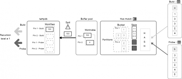
After the QP process all the rows from the probe input – the trick happens. Remember the spilled partitions, those written in Workfile into for the build and probe phases. Now, this data act like a new input into Hash Join, and the process is repeated from the step 1! Recursion.
Recursive hash joins
Hash Match starts from the in memory and spills partitions to the Workfile if necessary. If the spilled partition, after reading it from tempdb is still too huge to fit in memory, it splits one more time and the whole process goes to the deeper level of recursion and so on, until the partition will fit in memory.
We may observe the recursion level through in the actual plan warning section (from SQL Server 2012) or using Extended Events, or Profiler.
Bailout
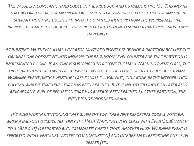
What if partitioning has no effect and the size of a partition remains the same, for example, there are a lot of duplicates, each and every time going to the same partitions increasing its size. From the certain point of recursion levels (I observed 5), that situation is considered to be a hash bail out. Meaning that a hashing algorithm is no more used for joining. Instead, a kind of loop algorithm is used comparing rows. This happens not for the whole input, but only for the overflow partitions, and this is a very rare situation. I’ve asked several people, if they had experienced hash bailout in real life and got a negative answer.
Role Reversal
If due to cardinality estimation error or bitmap filtering the probe side became smaller than the build side, Hash Match will reverse roles switching Build and Probe side. This behavior is known as Role Reversal.
In memory Example
After theoretical part, let’s do some action and observe how it works. We’ll start with a simple hash join that fit in memory. For the purpose of demonstration, I’ll create two rather big heap tables, 1 000 000 rows each. With the help of TF 7357 we will see some execution details.
Create test database.
|
1 2 3 4 5 6 7 8 9 10 11 12 |
use master; go if db_id('hashtest') is not null drop database hashtest; go create database hashtest go ---- set use hashtest; go create table Numbers(n int primary key); insert Numbers(n) select top(1000000) rn = row_number() over(order by(select null)) from master..spt_values v1,master..spt_values v2,master..spt_values v3; go |
Creating and filling the tables, and issuing the query
|
1 2 3 4 5 6 7 8 9 10 11 12 13 14 15 16 17 18 19 20 21 22 23 24 25 26 |
use hashtest; set nocount on; go if object_id('t1_big') is not null drop table t1_big; if object_id('t2_big') is not null drop table t2_big; create table t1_big(a int not null, b char(500) not null default('')); create table t2_big(a int not null, b char(500) not null default('')); insert t1_big with(tablockx) (a) select n%1000 from Numbers; insert t2_big with(tablockx) (a) select n%1000+1000 from Numbers; go dbcc traceon(3604, 7357) with no_infomsgs; dbcc freeproccache with no_infomsgs; go set statistics time, io, xml on; declare @a1 int, @a2 int; select @a1 = t1.a, @a2 = t2.a from t1_big t1 inner join t2_big t2 on t1.a = t2.a option(maxdop 1) set statistics time, io, xml off; go dbcc traceoff(3604, 7357) with no_infomsgs; go |
If we switch to the message tab, we’ll see a few interesting debug messages.
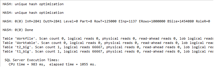
The first one, “Unique hash optimization”, is printed during the compile time. If you re-run the example with column “a” defined as nullable, then you won’t see this, but you will see the residual predicate property in the query plan, that means, that QP need to check this predicate also before concluding a match.
The second one is printed during the execution time and contains a couple of interesting things:
Level – recursion level
Part – number of partitions
RowT – estimated number of rows to fit each partition
ERows – estimated number of rows on the build side
BSize – bitmap size
RoleR – role reversal
This output is produced by the function CQScanHash::PickInputAndPrepareOutput, this function might correspond to logical step one in the algorithm described above, that means it is called at every recursion step and is very convenient to observe hash joining process.
Spilling and Bitmap Filters Example
Now let’s cheat QP simulating bad cardinality estimation with updating statistics with rowcount argument, to observe spill.
|
1 2 3 4 5 6 7 8 9 10 11 12 13 14 15 16 17 18 |
update statistics t1_big with rowcount = 1; update statistics t2_big with rowcount = 1; dbcc traceon(3604, 7357) with no_infomsgs; dbcc freeproccache with no_infomsgs; go set statistics time, io, xml on; declare @a1 int, @a2 int; select @a1 = t1.a, @a2 = t2.a from t1_big t1 inner join t2_big t2 on t1.a = t2.a option(maxdop 1) set statistics time, io, xml off; go dbcc traceoff(3604, 7357) with no_infomsgs; go |
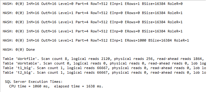
We observe several output lines, one line per iteration, for the last four lines recursion level is 1 and the Role Reversal behavior was involved – RoleR = 1.
Interestingly, there is a trace flag 7359, that disables bitmap filtering (step 14, 23). Lets’ do this with exactly the same query, to see what will happen, and how effective is bit-vector filtering.
|
1 2 3 4 5 6 7 8 9 10 11 12 13 14 15 16 |
dbcc traceon(3604, 7357, 7359) with no_infomsgs; dbcc freeproccache with no_infomsgs; go set statistics time, io, xml on; declare @a1 int, @a2 int; select @a1 = t1.a, @a2 = t2.a from t1_big t1 inner join t2_big t2 on t1.a = t2.a option(maxdop 1) set statistics time, io, xml off; go dbcc traceoff(3604, 7357, 7359) with no_infomsgs; go |
What we will see is:
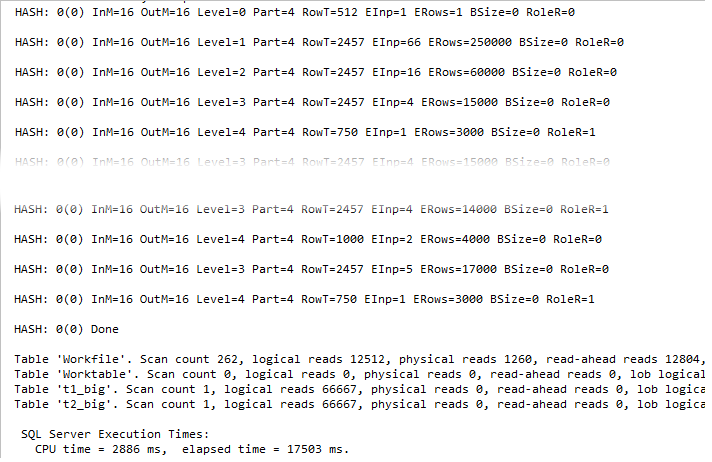
A few interesting notes about this output. First, the BSize = 0, i.e. there is no bit map. Persistent reader may check the invocation of the function CHashBitmap::Init in WinDbg. Without the TF 7359 it performs 510 instructions, doing some memory allocations and other actions, with TF enabled it returns in 14 instructions doing nothing.
Because of the disabled bitmap filtering, QP could not discard rows at the step 23,25, it should write to the probe Workfile every input row that corresponds to the spilled partition.
That means:
- No more reducing the probe side and the Role Reversal behavior occurs much more rare
- There are much more reads, due to the very intensive exchange with tempdb, and writes also (you may check it through sys.dm_io_virtual_file_stats dmv, my results are 16 MB vs. 109 MB written)
- There are much more joining steps and deeper recursion level, we may observe level = 4 here
- The time increased dramatically, almost 10 times
Bailout Example
I have never experienced a bailout situation in the real world queries, however, just for curiosity, I decided to reproduce it. For that purpose, we need tables with many duplicates, which will make partitioning technique not efficient. You can observe the bailout through Profiler or Extended events:
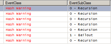
The above-mentioned TF allows seeing what kind of bailout it is. There are two of them: bailout and dual input bailout. The last one we will observe in action in the repro below.
|
1 2 3 4 5 6 7 8 9 10 11 12 13 14 15 16 17 18 19 20 21 22 23 24 25 26 27 |
-- Bail out if object_id('t1_big') is not null drop table t1_big; if object_id('t2_big') is not null drop table t2_big; create table t1_big(a int not null, b char(500) not null default('')); create table t2_big(a int not null, b char(500) not null default('')); -- %10 gives a lot of duplicates on both sides insert t1_big with(tablockx) (a) select n%10 from Numbers; insert t2_big with(tablockx) (a) select n%10 from Numbers; update statistics t1_big with rowcount = 10000, pagecount = 10000; update statistics t2_big with rowcount = 10000, pagecount = 10000; go dbcc traceon(3604, 7357) with no_infomsgs; dbcc freeproccache with no_infomsgs; go set statistics time, io, xml on; declare @a1 int, @a2 int; select @a1 = t1.a, @a2 = t2.a from t1_big t1 inner join t2_big t2 on t1.a = t2.a option(maxdop 1) set statistics time, io, xml off; go dbcc traceoff(3604, 7357) with no_infomsgs; go |
The output is:
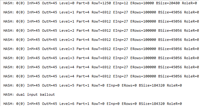
Dual input bailout at level 5. Also, notice the number of partitions before the bailout is considered – it is 1, meaning that partitioning gives no effect.
After preparing and publishing the article for the very first time, I have found a great article by Nacho Alonso Portillo from Microsoft about bailouts: What’s the maximum level of recursion for the hash iterator before forcing bail-out? This article explains the observed behavior about the recursion level 5 before a bailout, so I quote a related piece of information:
TF 7357 with Parallel Hash Join
Sharp-eyed reader may have noticed the MAXDOP hint in the test queries. It was placed there for two reasons: the simplicity of the query plan, and that TF 7357 does not produce output to console for the parallel hash join. However, it is still possible to see this in action. Add TF 3605 to direct output to the errorlog, and check it after the execution.
I used the following sequence of commands
|
1 2 3 |
dbcc errorlog; -- start new cycle for errorlog --run the query with option(querytraceon 8649) to force parallel plan exec xp_readerrorlog --read errorlog |
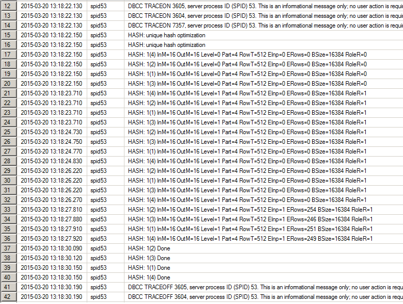
You may see the output in the errorlog, for precise information use the numbers that specify the Query Plan NodeID and Thread:
HASH: <NodeID>(<Thread>) …
Next article in this series:

Currently he works as a database developer lead, responsible for the development of production databases in a media research company. He is also an occasional speaker at various community events and tech conferences. His favorite topic to present is about the Query Processor and anything related to it. Dmitry is a Microsoft MVP for Data Platform since 2014.
View all posts by Dmitry Piliugin
- SQL Server 2017: Adaptive Join Internals - April 30, 2018
- SQL Server 2017: How to Get a Parallel Plan - April 28, 2018
- SQL Server 2017: Statistics to Compile a Query Plan - April 28, 2018