
Earlier this year, I published several articles on SQLShack with an aim of demonstrating tools available for visualising SQL Server 2017 graph databases. I was so caught up in the excitement of having SQL Server finally support graph databases that I forgot that some people still do not have a good grasp of how graph databases work let alone consider replacing their relational databases models in favour of graph. Although there are several ways that one can go about explaining the usefulness of graph databases over its relational counterpart, I have opted to focus on the benefits and strengths of graph databases by demonstrating the differences in which graph and relational databases deal with hierarchical datasets.
The Case for Hierarchical Datasets: Footballer-Manager Relationship
Hierarchical datasets are often synonymous with tree-like data structures and at one point or another, we’ve all been part of hierarchical data structures; be at places of work through employee-manager relationships, in our homes via child-parent relationships or through our levels of friendships on online social media platforms. The hierarchical relationship that I want to look at in this article is the Footballer-Manager relationship and how such a relationship can be represented in both graph and relational databases.
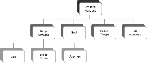
Figure 1 depicts a Footballer-Manager hierarchical relationship between players that – at some point – were part of the Spanish La Liga club, Atlético Madrid. As it can be seen in Figure 1, the majority of Footballer-Manager relationships are between manager Gregorio Manzano and players Gabi, Rubén Olivera, and Kiki Musampa. Whilst Diego Simeone was at some point managed by Gregorio Manzano, he has gone on to manage players of his own including the likes of Diego Costa, Gabi and Juanfran.

The information represented in Figure 1 can be modelled for both relational and graph databases. Consequently, I’ve gone ahead and produced such models as shown in Figure 2 wherein the left-hand side of the black vertical bar represents the relational database model whilst the other side represents the graph. Noticeably in both models is the fact that the FootballerManager entity has a relationship with itself – what is often called a self-join.
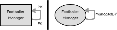
One significant difference in Figure 2 is the way self-joined relationships are indicated. For instance, keys are used in the relational model to denote relationships such that the foreign key links back to its primary key. Graph databases, on the other hand, take an entirely different approach to representing relationships. This is because, in graph databases, relationships are stored as standalone tables and thus the managedBY relationship is a standalone table separate to the FootballerManager entity. In other words, for every entity-relationship that you define in a graph database, a separate standalone table is created to store such a relationship. To demonstrate this argument, we’ve used information from Figure 2 to create a logical entity-relationship-diagram (ERD), shown in Figure 3. Again, the left-hand side of the black vertical bar in Figure 3 represents logical ERD for the relational database whilst the right-hand side signifies graph.
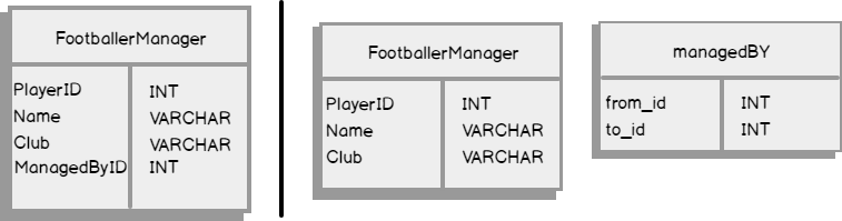
As per the total number of objects in Figure 3, graph database creates more physical objects than its relational counterpart. This means that we should expect the exercise of creating and populating objects in a graph database to be quite lengthier than a relational database. However – as it will be demonstrated later – all of your object-creation and populating efforts get rewarded later-on during data retrieval exercise as it is generally faster to retrieve hierarchical data out of graph compared to relational databases.
Measuring Query Performance: Relational Databases vs. Graph Databases
In this section, we compare query performances for both relational and graph databases by creating physical tables based on logical ERD design shown in Figure 3.
-
Measuring Relational Database Query Performance
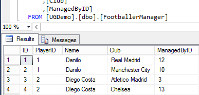
According to our ERD diagram for the relational database, we need to create only a single table – FootballerManager. I have gone ahead and created and populated such a table as shown in Figure 4 – (A database backup containing all tables used in this demo is available under the Downloads section at the bottom of this article).

Figure 4Having created and populated our table, we next move on to querying the table using Script 1.
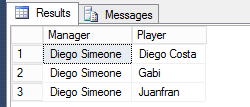
123456SELECT e.[Name] AS 'Manager',m.[Name] AS 'Player'FROM [dbo].[FootballerManager] e,[dbo].[FootballerManager] mWHERE e.[PlayerID] = m.[ManagedByID]AND e.[Name] = 'Diego Simeone';The results of Script 1 execution are shown in Figure 5 – which basically returns a list of all players managed by Diego Simeone.
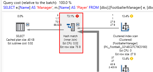
Figure 5Furthermore, using ApexSQL Plan I’ve gone ahead and generated an execution plan for Script 1. Notice in the generated execution plan in Figure 6 that the majority of Script 1 execution was spent performing hash match joins.
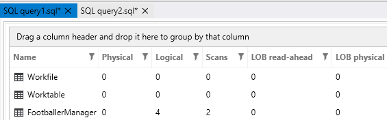
Figure 6 Hash match joins often indicate TempDB activity and as indicated in the query’s IO statistics shown in Figure 7, the SQL Server optimizer made use of Workfile and Worktable temporary objects to identify correct combinations that will satisfy query conditions stipulated in Script 1.
Figure 7 -
Measuring Graph Database Query Performance
Script 2 is graph database query version of Script 1.
1234567SELECT person1.name AS 'Manager',person2.name AS 'Player'FROM Footballer person1,Footballer person2,managedbyWHERE MATCH(person1-(managedby)->person2)AND person1.name = 'Diego Simeone';Script 2 The execution of Script 2 returns an output similar to what is shown in Figure 5 but as expected this version of the query in a graph database uses an entirely different execution plan to that of a relational database query.
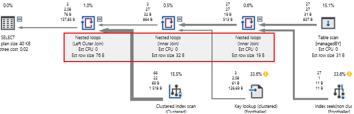
Figure 8 Figure 8 shows execution plan of Script 2. The execution plan indicates that the graph database query relied on nested loop joins instead of hash match joins used in the relational database version of the query. Nested loops basically identify matches by taking each record from the outer input and applying it against the inner input. In this case, our managedBY relationship table is the outer input being applied against the Footballer table. The predicate “Diego Simeone” reduces the size of our outer input from 27 to 3 – as 3 is the total number of records (relationships) linked to Diego Simeone. Now when we go looking for the names of the players linked to Diego Simeone, we only scan the Footballer table against 3 relationships instead of 27. So, the formula for our nested loop becomes 3*22 (number of possible player names) instead of 27 * 22.
Summary
Hierarchical datasets easily highlight the modelling and query execution differences in both relational and graph databases. However, this is by no means an indication that you should start throwing away the one database system over the other. Graph databases are more efficient when data relationships are at the core of your requirement. Below is a list of some key differences between Relational and Graph databases. We conclude this article by summarising some of the key differences between relational databases and graph databases.
| Relational Database | Graph Database |
| Entity Relationships exist as keys within dataset | Entity Relationships are represented as tables |
| Increase in size of dataset reduces query performance | Increase in connections/relationships degrades query performance |
| Harder to introduce new relationships/keys as it requires altering definition of underlying table | Easy to add new relationships |
Downloads
References
- Graph processing with SQL Server and Azure SQL Database
- Hash Match – SQL Server Graphical Execution Plan
- Hierarchical database model

Sifiso's LinkedIn profile
View all posts by Sifiso W. Ndlovu