Understanding Skewed Data in SQL Server

Introduction

I recently did some research to analyze skewed data distribution in SQL Server. This article is the outcome of my analysis to share with SQL Server community.

SQL Server understands its data distribution using statistics. The SQL Server query optimizer then uses the statistics to calculate estimated row counts when executing the queries submitted by users. The accuracy of estimated row count is crucial to get optimal execution plans. The SQL Server query optimizer is a complex mathematical component and it does a decent job to create better execution plans during a very short period of time.

However, getting better execution plans depends on the information that the query optimizer has. If the query optimizer has bad or insufficient information then it often results in suboptimal query plans which essentially leads to poor query performance which then leads to many other performance related issues in the database server.

Getting started

First, you need to download the sample data which I used for the demo scripts as well as the stored procedure named, analyze_skewed_data from the link provided below.

Please use this link.

Note: All the demo codes are tested in SQL Server 2016 SP1 CU2 (13.0.4422.0). I use some features which are available in SQL Server 2016 and above.

Use the following code to create a new database called, SkewedDataDB and a new table called, bigtable.

USE master;

CREATE DATABASE [SkewedDataDB];

--So that I do not have to worry about t-log getting full.

ALTER DATABASE [SkewedDataDB] SET RECOVERY SIMPLE

USE [SkewedDataDB];

--Create a new table.

DROP TABLE IF EXISTS dbo.bigTable;

CREATE TABLE dbo.bigTable

(

bigTable_id int IDENTITY(1,1) CONSTRAINT PKC_bigTable_id PRIMARY KEY,

id_1 int,

id_2 int,

id_3 int

);

Download the zip file, filtered_stats_bigtable.zip using the link mentioned above. Refer the README.md file for more details.

Then, use the following code to load the initial data and then insert the same data set again to make skewed distribution.

Note: Change the path to point to the text file you just downloaded.

BULK INSERT dbo.bigTable

FROM 'D:\Temp\bigtable.txt'

WITH (FIELDTERMINATOR = ',', ROWTERMINATOR = ';')

Output:
(9604608 row(s) affected)

--insert more data to create skewed data distribution.

INSERT INTO dbo.bigTable (id_1,id_2,id_3)

SELECT id_1,id_2,id_3

FROM dbo.bigTable

GO 2

Output:
Beginning execution loop
(9604608 row(s) affected)
(19209216 row(s) affected)
Batch execution completed 2 times.

After executing the preceding query, the bigtable should have more than 38 million rows. Since the same data set is inserted twice, it creates a skewed distribution.

You can check the exact row count of the table using the following code.

SELECT OBJECT_NAME(object_id) TableName,SUM(rows) Row_Cnt

FROM sys.partitions p WITH (NOLOCK)

WHERE object_id = object_id('dbo.bigtable')

AND p.index_id < 2

GROUP BY OBJECT_NAME(object_id)

Exact row count is: 38,418,432

At this point, the data set is ready. Let’s create a non-clustered index on id_1 column before we execute some queries against this column.

CREATE INDEX ix_id_1 ON bigTable (id_1)

Execute sample queries

Let’s execute the following three queries with Actual Execution Plan being enabled. You can use CTRL + M to enable the Actual Execution Plan.

SELECT * FROM dbo.bigtable

WHERE id_1=3882

Output:
(0 row(s) affected)

SELECT * FROM dbo.bigtable

WHERE id_1=38968

Output:
(4 row(s) affected)

SELECT * FROM dbo.bigtable

WHERE id_1=9744

Output:
(23912 row(s) affected)

See the Graphical Execution Plans of the preceding three queries below in sequence.

Figure 1: Graphical Execute Plans of three queries

You might be wondering about the, “missing index” warning even though the column, id_1 has an index. However, in this case, missing index hint is for the covering index. So please ignore the warning since it is not related to our discussion.

Estimated number of rows

If you hover the mouse pointer to Index Seek operator in any of the three execution plan(s) mentioned above you would see something like below;

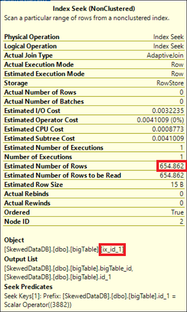
Figure 2: Properties of Index Seek Operator

If you check the Estimated Number of Rows of the Index Seek operator in all three execution plans, it will be 654.862. See below table for the comparison of Estimated vs Actual row count of the query executions stated above.

Query	Estimated Number of Rows	Actual Number of Rows
Query 1	654.862	0
Query 2	654.862	4
Query 3	654.862	23912

Table 1: Estimated / Actual Row counts before the filtered stats.

As you know, SQL Server query optimizer uses statistics to determine the cardinality estimation, in this scenario, the query optimizer has used the histogram information of the statistics of the index, ix_id_1.

We can verify it by observing the histogram of the ix_id_1.

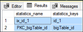
Let’s check all the statistics available for the table.

EXEC sp_helpstats 'dbo.bigTable','all'

Output:

Figure 3: All the stats related to bigtable.

Let’s look at the histogram of the index, ix_id_1.

First, you need to get the stat id of the statistics object. You can use the following code for that.

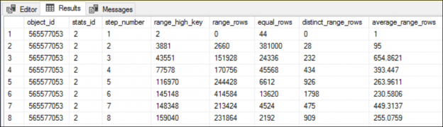
SELECT [name], stats_id, filter_definition

FROM sys.stats WHERE object_ID=OBJECT_ID('dbo.bigtable');

SELECT * FROM sys.dm_db_stats_histogram (OBJECT_ID('dbo.bigtable'),2);

Note: The DMV, sys.dm_db_stats_histogram is new to SQL Server 2016. It has been introduced in SP1 CU2. So, in case you do not see this DMV in your SQL Server, please double check the latest patch level, and install SP1 and CU2. This DMV comes handy when you want to further analyze the histogram programmatically. Alternatively, you can use DBCC SHOW_STATISTICS command as well but you need to get the result into temporary table and then join with other tables. So, it’s a little bit of extra work there.

DBCC SHOW_STATISTICS (bigtable,ix_id_1) WITH HISTOGRAM;

The predicate values we have used in the preceding queries are, 3882, 38968, and 9744 respectively. If you look at the histogram of the index, ix_id_1, you will notice that all these three values are between the RANGE_HI_KEY 3881 and 43551.

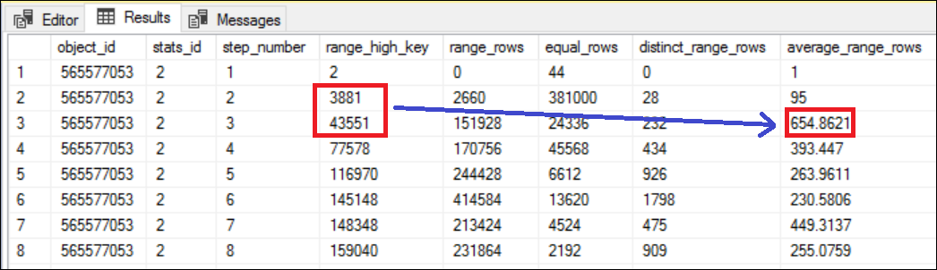
Figure 4: The Histogram of the index ix_id_1

The average range rows between the steps 2 and 3 (which is essentially between the RANGE_HI_KEY 3881 and 43551) is 654.8621. See Figure 4 for more details.

The number 654.862 is equal the Estimated Number of Rows in the Index Seek operator of the all three execution plans. Literally, if you specify any value between the RANGE_HI_KEY 3881 and 43551, SQL Server query optimizer estimates the row count as 654.862 and no matter how much actual number of rows returned by the query. This is based on the statistical understanding of the data distribution in column, id_1.

Data distribution

We can analyze the actual data set between the steps (2 and 3) in the histogram mentioned above. Use the following query to extract all the rows and aggregate the data for the index column, id_1.

SELECT id_1,COUNT(*) AS nof_rows FROM dbo.bigtable

WHERE

id_1 > 3881 and id_1 < 43551

GROUP BY id_1

ORDER BY 2 DESC;

Output:
(232 row(s) affected)

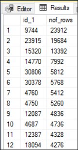
Figure 5: Top 12 records of the aggregated row count for id_1 column between the values 3881 and 43551.

Within the range, there are 232 unique id_1 values and each value has the total number of records as shown in the Figure 5. The highest total number of records is 23912 and the lowest being 4. However, according to the statistical understanding of the data, SQL Server always estimates the row count as 654.862 which is the average number of rows between the two steps. When we compare the value 654.862 with the actual number of rows returned, it is not even close for some cases.

The query which process 4 records is different to the query which process 23912 records in terms of resource utilization. The reason that you see a significant gap in estimated and actual number of rows is because of the skew data.

Filtered statistics

What if you manually create a statistic for the steps 2 and 3 of the histogram in Figure 4. Let’s create the following statistics and execute the same three queries again. Since we create the statistics with WHERE clause, it is called filtered statistics. Filtered statistics was introduced in SQL Server 2008.

CREATE STATISTICS id_1_3881_443551 ON dbo.bigtable (id_1)

WHERE id_1 > 3881 AND id_1 < 43551

WITH FULLSCAN

Creation of a statistics is very light weight process unlike an index creation it does not consume lot of server resources. Execute the queries again and check the estimated and actual number of rows in Index Seek operator. See Table 2 for more details.

Query	Estimated Number of Rows	Actual Number of Rows
Query 1	1	0
Query 2	4	4
Query 3	23912	23912

Table 2: Estimated and actual row counts after the filtered statistics.

The results are very interesting. After creating the filtered statistics, the query optimizer has been estimated the row count very accurately. You will know how SQL Server has processed the row estimations by looking at the histogram information of the filtered statistics we just created.

SELECT * FROM sys.dm_db_stats_histogram (OBJECT_ID('dbo.bigtable'),3);

Note: 3 is the stat id of the filtered stat.

How to identify Skewed Data in your table

To create filtered statistics to address the skewed data issue, you need to identify the step(s) of the histogram that needs filtered statistics. Analyzing it manually would be a cumbersome task. So, I created a stored procedure which accepts a table name and a stat id as arguments and analyze the data by calculating standard deviation (SD) and coefficient of variation (CV).

Note: This stored procedure is still in beta version. So be extra careful when you run this in production for very large tables (VLT). Appreciate your feedback on this and any improvements that you think is necessary.

Download the stored procedure (analyse_skewed_data) and create it, in the database.

EXEC analyse_skewed_data 'bigtable',2

Output:
(188 row(s) affected)

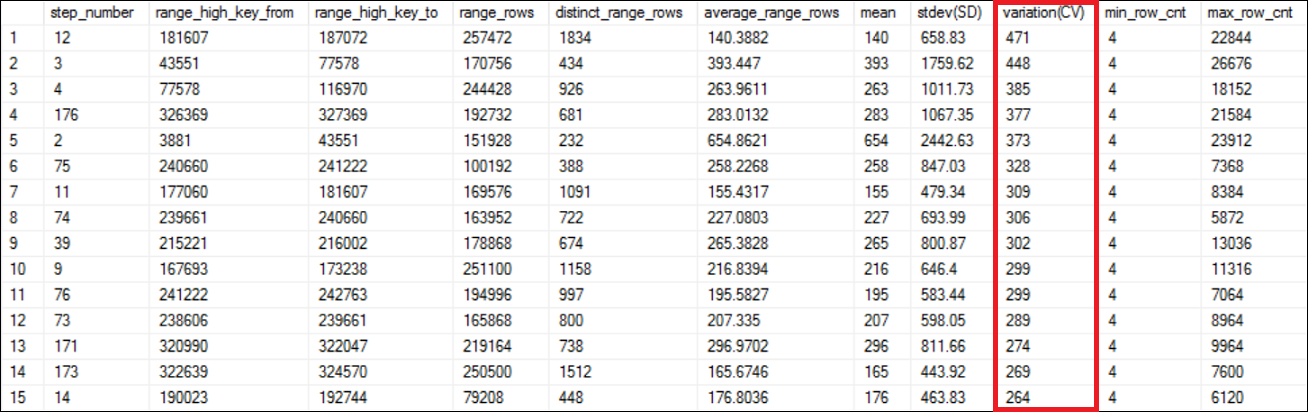
Figure 6: Top 15 records of skewed data analysis result.

Understanding Skewed Data analysis result

As shown in Figure 6, the result is ordered in descending order of the variation (CV) column. The range_high_key_from, range_high_key_to, range_rows, distinct_range_rows and average_range_rows are directly from the histogram of the statistics being analyzed. Explaining those information is out of scope of this article.

The mean column is same as average_range_rows except it is an integer. The mean, is calculated as below;

Mean = range_rows / distinct_range_rows

The standard deviation, stdev (SD) is the most important column in the result. The SD is a measure of spread of the data. It tells you, how much the data varies from the average (mean). The higher the SD, the higher the variation (CV) too. In other words, if you have more skewed data, you will see higher values in the variation (CV) column.

The variation (CV) column is calculated as below;

Variation(CV) = stdev(SD) / mean * 100

In statistical terms, the variation means, the ratio of standard deviation to the mean. Higher values in variation means, skewness of the data is also high. The variation is also called as the coefficient of variation (CV).

Look at the data range we have used for the preceding queries. The step range is 3881 and 43551 which is the 5th highest skewed data range according to the Figure 6. Now you can decide which step ranges that you probably need to create filtered statistics to address the skewed data issue so that the optimizer could estimate the row count accurately.

Let’s analyze the newly created filtered statistics to see whether we have successfully addressed the skewed data issue. I expect the very low values for the variation (CV) column this time. See Figure 7.

You can notice the stat id of the newly created filtered statistics object is, 3.

EXEC analyse_skewed_data 'bigtable',3

Output:

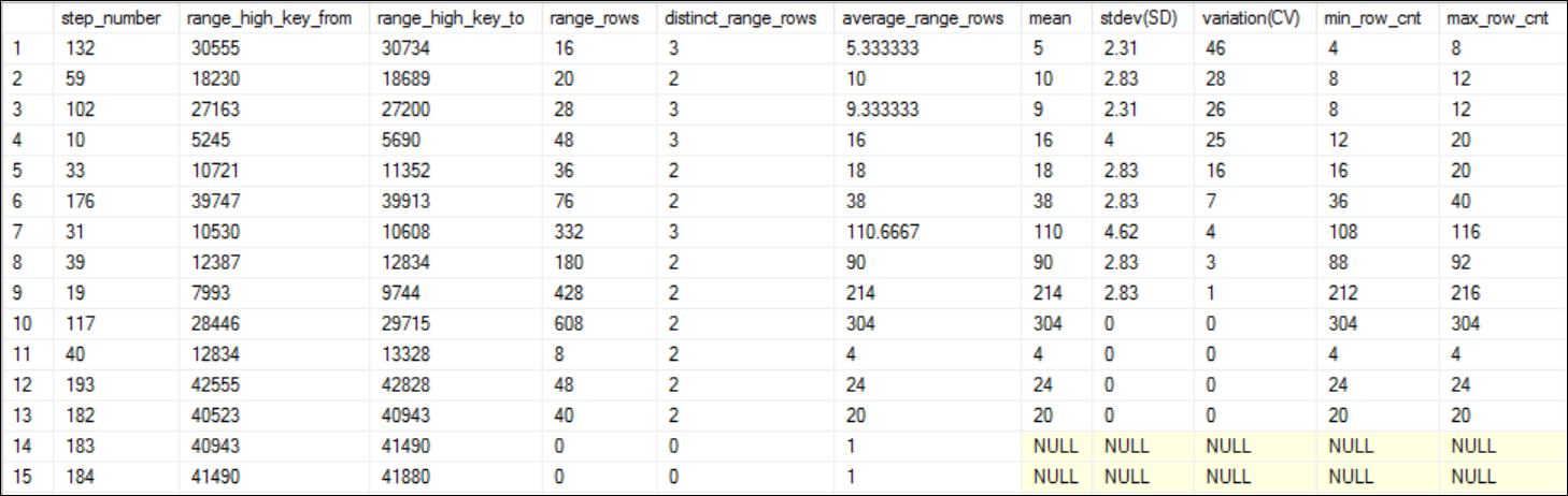
Figure 7: Top 15 records of skewed data analysis result with filtered stats.

Look at the variation(CV) column and see all the values are less than 50%. You can observe series of NULL values as well for variation(CV) column, which essentially means, it cannot calculate the coefficient of variation because the average range rows are, 1. In statistics what it means, to calculate the SD you need to have more than 1 observation. Since average range rows is 1 means you have a single observation meaning the SD is NULL then CV is also NULL. If you consider skewed distribution, if the SD or CV is NULL means, the data is not skewed.

Summary

You can influence the SQL Server query optimizer in various ways including index hint. However, in this scenario we did influence the query optimizer in a good way which is creating additional statistics to address skewed data. We also covered the steps to identify skewed data in a table so that you can consider creating filtered statistics to improve the cardinality estimation.

Downloads

Analyze_skewed_data

Author
Recent Posts

Susantha Bathige

Susantha Bathige (MSc, BCS, MCSA, MCITP) is a Microsoft Certified database professional specialize in relational database product, Microsoft SQL Server. He has more than 16 years of IT experience including more than ten years in database development and administration in non-production and production environments. He has experience of other databases systems such Cassandra and MongoDB as well. Blogs: http://www.sqlservertorque.net/ and http://www.databasetorque.com/

Latest posts by Susantha Bathige (see all)

Understanding Skewed Data in SQL Server - May 22, 2017

Introduction

Getting started

Execute sample queries

Estimated number of rows

Data distribution

Filtered statistics

How to identify Skewed Data in your table

Understanding Skewed Data analysis result

Summary

Downloads

Related posts: