Basics of TOP Operator

The TOP keyword in SQL Server is a non-ANSI standard expression to limit query results to some set of pre-specified rows. As an argument, it takes 0 to positive Bigint (9223372036854775807) and anything beyond or less gives an error message. TOP without an order by clause, in production, seems buggy because it can produce results in any order depending on the current schema and execution plan. You can also specify a percent with TOP expression which returns only the expression percent of rows from the result set. Float expressions used in TOP percent are rounded up to the next integer value.

Deterministic TOP with order by (TOP With TIES)

TOP is only deterministic when order by is specified. Only then you can guarantee the result will be in a certain specific order. But even a TOP with order by can be non-deterministic when order by column(s) contains non-unique values.

Consider a scenario a user come with a requirement of TOP 3 product performed best in sale for the given saledata:

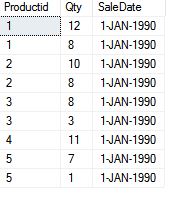
If you look at the data above, ProductID 3 and ProductID 4 aggregated sale Quantities are equal to 11.

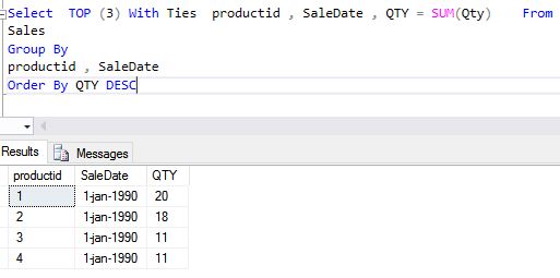
So actually both qualify for the 3rd place, but With regular TOP with ascending order by only 1 will be chosen randomly, of course, there are many ways to fulfill the requirement, but SQL Server has TOP with Ties which is useful when you want to return two or more rows that ties for last place in the limited results set.

Below is the result of above data of query TOP (3) with ties, as we can see that 4 rows are in the below result set as ProductID 3 and 4 qualify for the 3rd place.

Sample Data

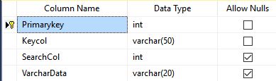
We will use two tables, table1 and table2 for the example below in this article. Table2 is just a replica of table1, so both tables have the same data and data type. Both tables have 300000 rows. The primarykey column is marked as Primary Key.

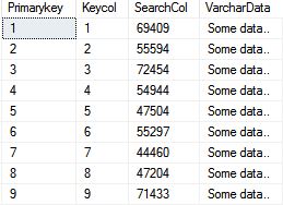
The primarykey and Keycol column consists of a numeric sequence from 1 to 300000 and the searchcol column has some random data. Below are the images of sample tables and the data.

You can find the script to populate the data from below of the article.

Testing Environment

Microsoft SQL SERVER 2014 – 12.0.4100.1 (X64) Developer Edition (64-bit)
Microsoft SQL SERVER 2016 (SP1) – 13.0.4001.0 (X64) Developer Edition (64-bit)

Table/Index scan with TOP 1

The Table/Index scan is usually misunderstood by SQL Server users as it touches all the data pages of Table/Index. Sometimes it’s not at all necessary to touch all the rows from the table/index scan, for example, a semi-join or when you set the row goal. In both cases, it’s not necessary to touch all the data pages. Execution can terminate early when it founds the requested row.

As stated above, with non-deterministic TOP expression queries, it sets up the Row Goal to return the N number of rows and it doesn’t matter in which order, so it’s completely unnecessary to get all the data pages. Just get an N number of rows and return it to the SSMS result tab.

I will run dbcc dropcleanbuffers to flush all the data pages. Please note that the dbcc dropcleanbuffers command is not recommended on a production server .

Look at the query below with STATISTCS IO ON you will get the idea.

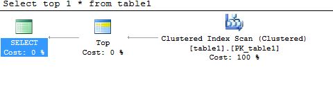
Table ‘table1’. Scan count 1, logical reads 3, physical reads 3, read-ahead reads 0, lob logical reads 0, lob physical reads 0, lob read-ahead reads 0.

The Execution plan shows, on the right side, its clustered index scan strategy used to fetch the data from the table. Now look at the output of STATISTICS IO and you can see that there are just 3 logical reads. This verifies, for the above execution, that on the query index scan hasn’t read all the data pages from the index. It looked for only 1 row and when it finds it, it stops looking further.

How an Execution plan reads (Row mode)

In SQL Server, an execution plan’s operators are called iterators for the reason that they work repeatedly like an iterations and process row by row based on demand-driven pipeline model.

Generally, there are three common functions called by iterates:

1 OPEN: to initialize the iterator.

2 GETNEXT: get the row and process according to the iterator property.

3 CLOSE: Shut down the iterator.

Execution starts from the leftmost iterator and control passes to next iterator, data flow to right to left.

The TOP iterator helps it to understand how the execution plan runs left to right not right to left. To understand it better we will execute a query with TOP expression and examine an execution plan. Warm the cache by running the below query ones at least.

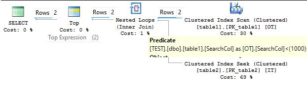
Execution starts from the leftmost select iterator, then control passes to TOP iterator.

In the above execution plan TOP expression 2 is used that set up the row goal for 2 rows, then control passes to nested loop join iterator, then table1(clustered index scan) initiated and starts requesting the data for the filter ([TEST].[dbo].[table1].[SearchCol] as [ot].[SearchCol]<(1000)) on the Table1.

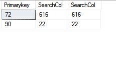
The first row that satisfies the filter criteria is 616 (the result would vary on your system). It is associated with the primarykey column value 72, so the nested loop join initiated the search for the value 72 in the table2, as table2 is indexed on the primarykey column so seek happened and passed all the request column to the nested loop join iterator. The nested loop join gets the data and sends it to TOP iterator and TOP iterator passes it to select an operator, then again filtered applied on the Table1(Cluster Index Scan) and return the data to the nested loop join then it matched to the Table2 then return the matches to the TOP iterator. Because only 2 was specified in the TOP expression, it signals to shut down to nested loop join and that signal is passed to both the outer and inner tables.

However, on my system for the predicate [ot].[SearchCol]<(1000) there are 3077 actual numbers or rows present in the table, but because execution follows demand-driven pipeline model, the nested loop join iterator produced only 2 rows to the TOP iterator and shut down scanning when parent iterators signal it to shut down.

Please note result may vary to your system as the above query results are non deterministic. If you want to explore more about it you can see this link SQL Server query execution plans – Understanding and reading the plans.

TOP 1 problem with aggregation and parallel nested loop join

In this part of the article, we will see a specific situation with TOP 1 where Query Optimizer final selected plan runs extremely slow. We will try to examine the Query Optimizer final cheapest selected plan for the below expressed query and is it really scale and perform well if not, then we will try to find out the reason behind it and available alternative if this pattern bothers you.

Consider a scenario where you need to count number of occurrences of maximum numeric value in the searchcol column of table1 after joining the table2. What if you have this task in hand and you have to do it manually how would do it? Most probably the answer would be:

Get both inputs

Step 1: join two inputs

Step 2: Group the output result on search column

Step 3: order by column descending

Step 4: get the TOP 1

There are many alternative options are available to express the above requirement in the query, but most natural seems to me has written below. Now lets see how it implements by the Query Optimizer with an estimated execution plan query and execution plan below:

Step 1: Get the Table1

Step 2: Sort table 1

Step 3: join table 2 (stream based non blocking) with nested loop join

Step 4: group the output result

Step 5: get the TOP 1

More detail description below: (we will debug this as data flow perspective)

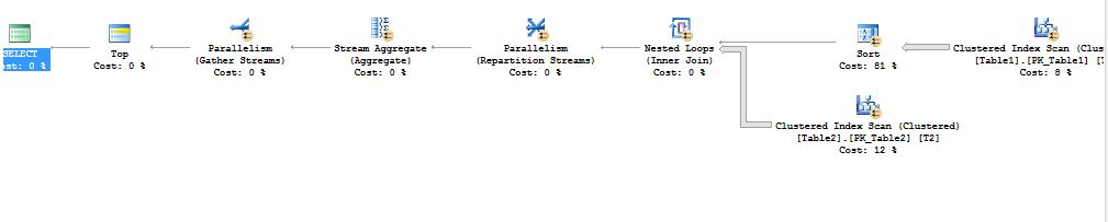
The Query Optimizer chooses a parallel execution plan. The chosen technique is actually a very smart approach for the two large tables (the Query Optimizer only join 2 tables at a time, if in the query there are more than 2 tables, then the join tree of tables is purely cost based).

As for the above expressed query there is no need of joining all the rows, so it’s wise to just sort one input (here the Query Optimizer is using a full outer table sort after all the outer side rows are sorted then passes to the nested loop join row by row on demand) as specified in the order by clause then display the output.

This kind of implementation, with a non-blocking loop join, suits best as it would preserver the outer order (in some cases NL doesn’t preserver the outer order, but here it will preserver the outer order) and then group with global stream aggregated (it requires the same set of values at same the worker thread, somehow its child iterator responsibility to do that, it’s not blocking but required sorted input) and pass the sorted first group to the TOP iterator.

Now let’s run the query with Maxdop 2 to limit the query for and turn on the actual execution plan:

Something went really wrong as it took 1:13 minutes to complete the execution on my system, so what was wrong in the above execution. Maybe we are running with Maxdop 2. Let use maximum capacity of system CPU processing and check how much query performance improved.

Here it took 3:56 minutes to complete the execution. If your machine has more than 4 processors, then try to run it with the maximum logical processor available. If your query is having the same pattern, then I am sure it would be worse by increasing of DOP. We are using a machine with four logical processors available to SQL Server.

Why would this query execution time become worse with increased DOP? Does that mean parallelism is bad?

Not at all. Parallelism is a boon in SQL Server and itself implemented very well. SQL Server uses horizontal parallelism for every iterator. Each worker is assigned a separate part of the work and the partial results are combined for the final result set. For queries involving large datasets SQL Server generally scales linearly or nearly linearly.

So let’s go back and try to understand why query took that much time execution plan below:

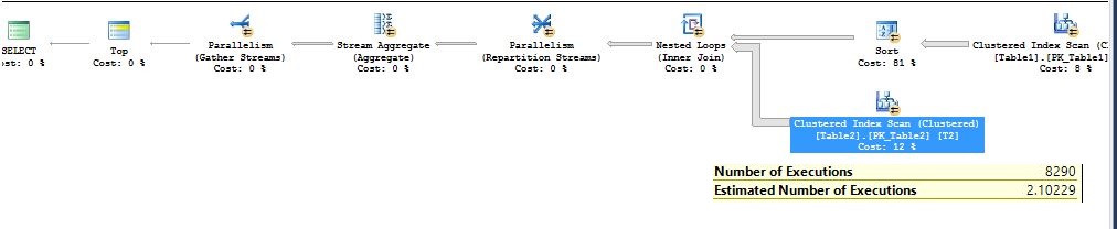
You can see that the number of executions at the inner side for the table2 of nested loop joins its 8290 and the estimated number of execution is 2.10229. That means that the Query Optimizer comes with this final execution plan with nested loop join because it estimated that nested loop join will only be executed to near about 2.10229 times but it actually executed 8290 times on my system. Keep in mind that both tables have perfect statistics in place. Still, we are seeing a huge difference in an actual VS estimated number of executions.

So finally, it turns out that the Nested Loop Join is the main culprit for the slow performance of the query.

As Stated above TOP, SET ROWCOUNT, Fast N and IF EXISTS enable the row goal and this change the optimization model to generate the query plan for specified rows only, in some specific cases, After enabling the row goal the query may take a long time to run. Microsoft is aware of this problem so there is a TRACE FLAG 4138 to disable the row goal. Let’s run the above query with this trace flag and see the actual execution plan.

It uses the same steps as we expected in the very first guess:

Get both inputs

Step 1: join two inputs

Step 2: Group the output result on search column

Step 3: order by all descending

Step 4: get the TOP 1

More details:

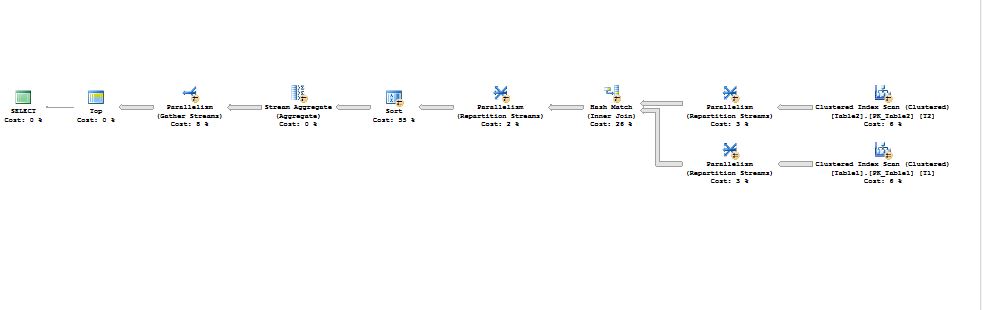
The Query Optimizer again chooses a parallel execution plan, as no predicate was specified in the query.

Here is the sequence of operations

• The entire table2 is build input for the hash match,
• Rows are then distributed to all the available threads on demand based schema by the Parallel Page Supplier,
• Then exchange iterator (hash iterator, we will give details about hash exchange iterator later),
• Then hash Match (Hash joins parallelize and scale better than any other physical join type and are great at maximizing throughput in data warehouses) is applied, as a physical join type as the hash join is a blocking iterator for the build input and it required additional memory to build the hash table in memory.

Note that this may spill into tempdb if not enough memory available for hash join at a run time. One tip we should remember while dealing with parallel hash join is that memory is divided amongst the threads equally, so a hash join can spill even if enough memory calculated for the hash join but rows skewed across the threads for any reason.

However, this is not the case in the above example, as rows are evenly distributed amongst the threads and hash join ran entirely in memory, as shown in the execution plan global stream iterator used for aggregating the rows (because before joining the two table hash partition applied which is deterministic function which guarantees that values don’t overlap between the threads) and the estimated cost calculated for this version of execution plan is 22.5983 units, the memory grant to this query on my system is 83.328 MB and it ran for 583 ms only. As such this was quite an improvement without any index.

Let’s go back to the first query which chooses the nested loop join, and try to deep dive and understand the execution plan.

Both tables used in the query are identical and represent the same dataset, so why did it take that much time and after increasing the maxdop setting and why is it worse?

This time we will use the DMV sys.dm_os_waiting_tasks for more detail information. We will run our queue and on the other session we will run the dmv and try to interpret its result.

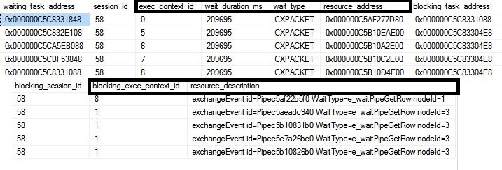
The DMV shows Execution Context ID 5 to 8 blocked on a CXPACKET wait by Execution Context ID 1 and Execution Context ID 0 blocked on a CXPACKET wait by execution context 8. Execution context zero is a coordinating thread that runs the serial part of the execution plan to the leftmost Gather Streams operator. CXPACKET (Class exchange packet) means that the thread is involved in a parallelism-related wait. You can find more details in the resource_description column for Execution Context ID 5 to 8 it says Node ID 3 is waiting to get rows, looking into the execution plan confirm node id 3 is exchange iterator (hash partition).

So now let’s deep inside exchange iterator:

The Exchange iterator is unique in many ways as it’s quite different compared to other iterators, It is actually two iterators: a producer and a consumer. The producer reads input rows from its branch and pushes data to the consumer side of exchange iterator, whereas most iterators follow the Demand-driven model. Data flow between exchange’s producer to consumer iterator follows the push-based method for efficiency reasons. It fills the packet with rows (that’s why parallelism iterators always required additional memory) and passes it to the consumer side. The consumer side receives packets, removes the rows from these packets, and returns rows to its parent iterator based on demand-driven pipeline model. One important detail that needs to be understood here is that the packet of rows at the producer is only transferred when a packet is full or a child iterator runs out of data.

Now look at the execution plan again and now more specifically at node 3 as reported above by the sys.dm_os_waiting_tasks dmv. Node ID 3 in the above execution plan is the parallelism (exchange) iterator. Parallelism (exchange) iterator with hash partition type routes incoming rows to the all available threads using a hash function (deterministic) on the partition column. So rows won’t get mixed up with other threads, in our query partition column is searchcol column.

From the child iterator (nested loop join) parallelism iterator gets 8484 rows, but passed only 45 number of rows to the parent (stream aggregated) iterator, for the reason as stated above. The exchange iterator’s producer side sends rows to the consumer in a packet only, when either packet is full or the child iterator runs out of data, so producer side of parallelism iterator waited for nested loop join to fill the data packet. When the data packet filled with rows then it send to consumer side of parallelism iterator, the consumer side of the exchange receives data packet(s) and removes rows from the packet(s) and then send it to its parent iterator (stream aggregated) based on demand.

So if somehow we would able to reduce the packet size (not possible) at the producer end of exchange iterator or increase the searchcol column data size, then the producer side would send the packet to the consumer side early. Here we will do a small test to fill the producer of the exchange early by altering the data type at the run time to the maximum capacity of numeric data type per row, so the exchange packet could fill up early and send the packet early.

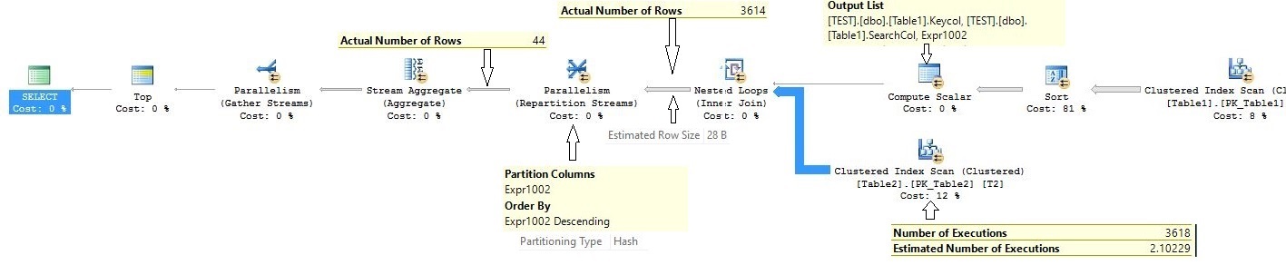
The execution plan shape is identical to our first parallel nested loop join query. There is just one additional compute scalar iterator after the sort iterator, a compute scalar has a task to convert the integer searchcol column to decimal, and the new value is labeled as [Expr1002].

Now note that the Exchange (parallelism) iterator partition type is also Hash type and partition column is [Expr1002]. The actual number of rows feeding to exchange iterator is 3614 whereas in the last query actual number of rows were 8484. It happened because now the producer side of the exchange is able to push the data packet to the consumer side of exchange early because the row size is now increased. Hence the data packet filled up with a few rows and pushed an early compares to the last execution plan. This query executed in 1:40 minutes on my system.

As stated, for the problem, specific to the above, with this data set nested loop join would be the best strategy. We need to eliminate exchange (parallelism) iterator from the query plan, so we will run again the query with maxdop 1 to force SQL Server to choose the serial version over its default parallel version of execution.

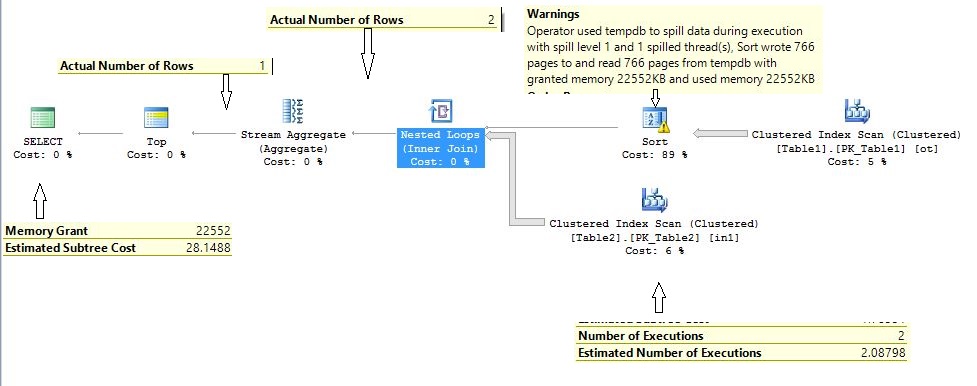
If you are running this query on SQL Server 2012/2016, you might see the sort is spilling to the tempdb as reported on my system. It states “Operator used tempdb to spill data during execution with spill level 1 and 1 spilled thread(s), Sort wrote 766 pages to and read 766 pages from tempdb with granted memory 22552KB and used memory 22552KB”. This is strange as the estimated number of rows and average row size are accurate, and the system has sufficient memory still it spills to the tempdb.

Actually, it is a bug in SQL Server which appears in certain conditions and it is fixed in subsequent updates. To enable this fix you need to use the trace flag 7470, however, this trace flag should not be enabled at the server level as it increases memory requirements for sort queries and may impact memory availability for concurrent queries.

Apart from that, as expected, the plan is identical to parallel nested loop join. This is a perfect looking plan shape as the inner side on nested loop join executes twice and passed 2 rows to the stream aggregated and more importantly the query executed in 273 milliseconds.

I have seen these parallel nested loop join with row goal running for a long time and consuming all the CPU resources. it doesn’t run itself slowly but affects other concurrent queries as well, competing for resources. I hope in this article we all get the idea how row goal can affect your query performance and how to deal with it.

Here you can download a script to populate the Sample table.