
Introduction
In a past chat back in January 2015, we started looking at the fantastic suite of data mining tools that Microsoft has to offer. At that time, we discussed the concept of a data mining model, creating the model, testing the data and running an ad-hoc DMX query. For those folks that may have missed this article, the link may be found immediately below;
Grab your pick and shovel and lets mine
In the second part of this article, we shall see how we may utilize the information emanating from the models, in our day to day reporting activities.
So grab that pick and shovel and let us get to it!
Getting Started
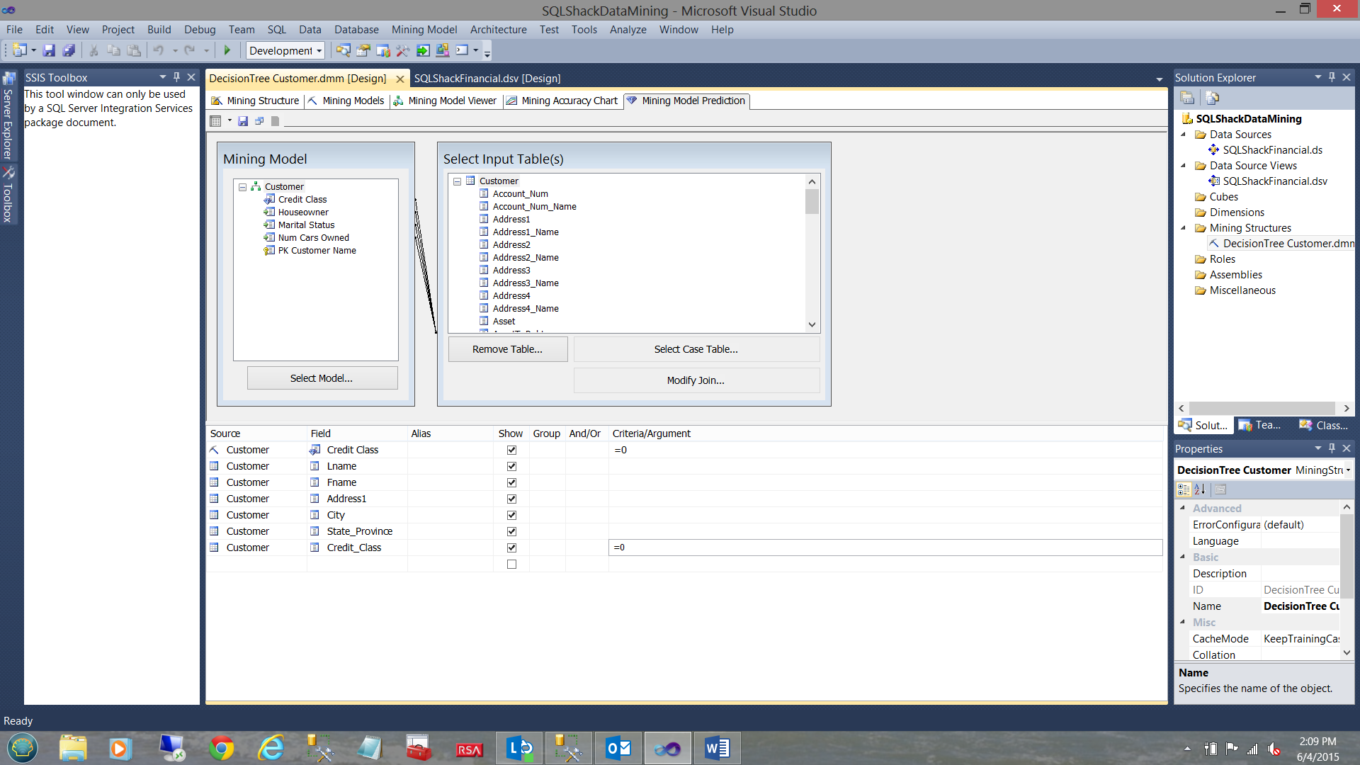
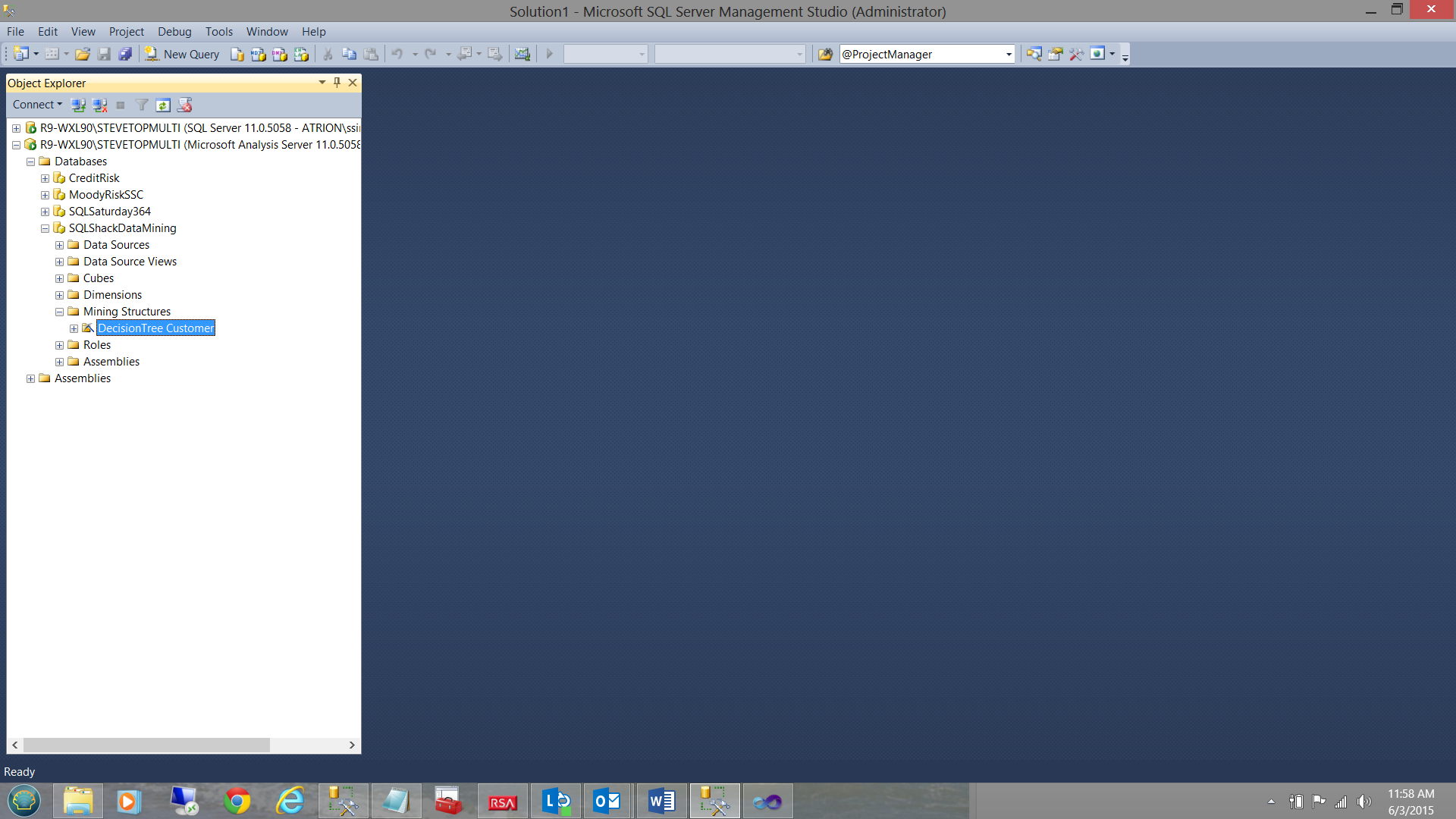
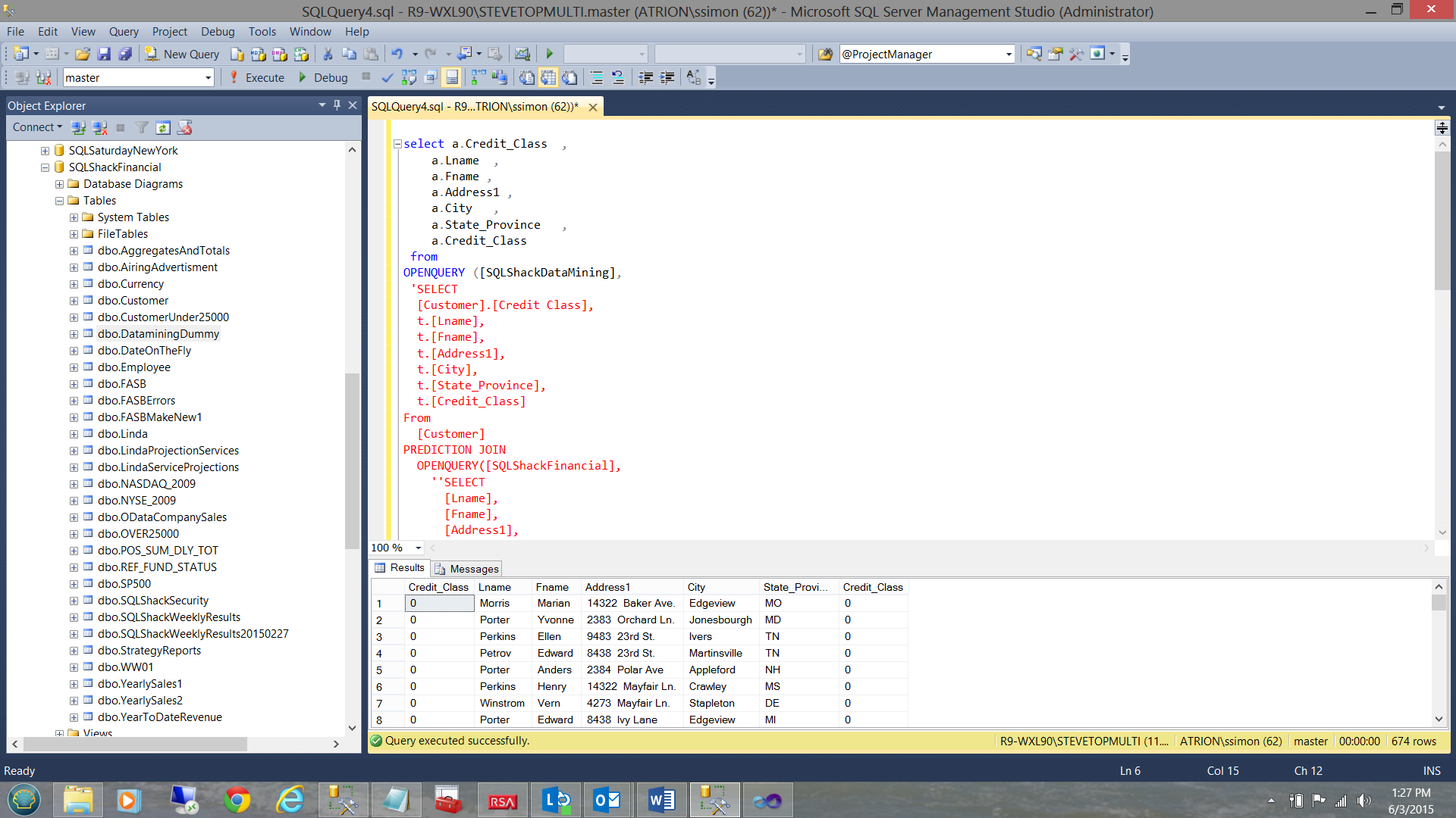
Based on the final screenshot of the first article (please see the hyperlink above) we are going to pick up from here with SQL Shack’s newest data (which came in this morning) and we are going to utilize the model that we created back in January 2015 to see how valid our model is, against the newest data.
The reader will note that we have selected the mining model prediction of ‘a great credit class’ i.e. 0 (see the highlighted cell above) and we are going to pit this against the data from the newest data table “Customers”.
In order to validate our results, we set the mining model predicted credit class to 0 and the actual “Customer” credit class (from the credit agencies) to 0 as well (see above).
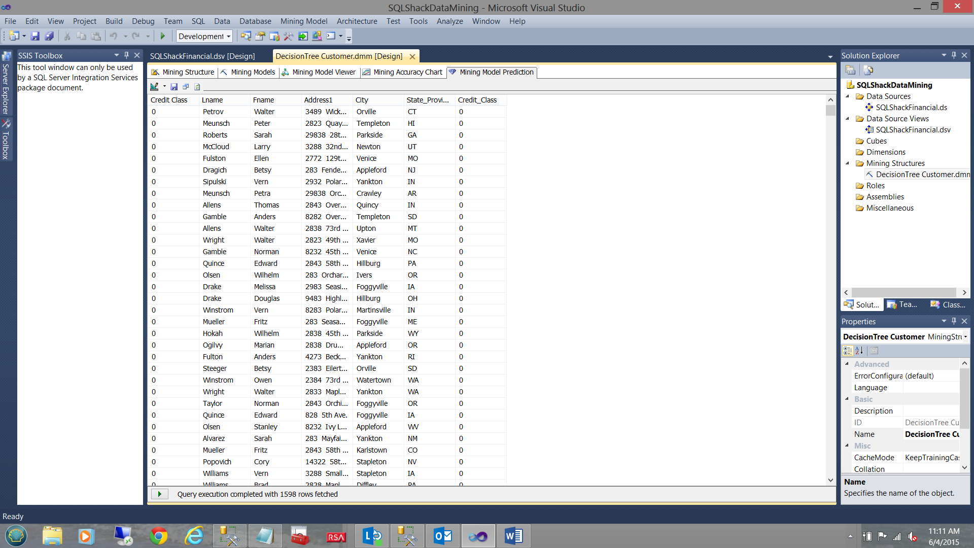
The results of the query are shown above and we note that these are the folks that are probably a safe credit risk. 0 being the best credit class.
The astute reader (of the first part of this article) will have noted the similarities of the screenshot shown above and the last screenshot of the January article.
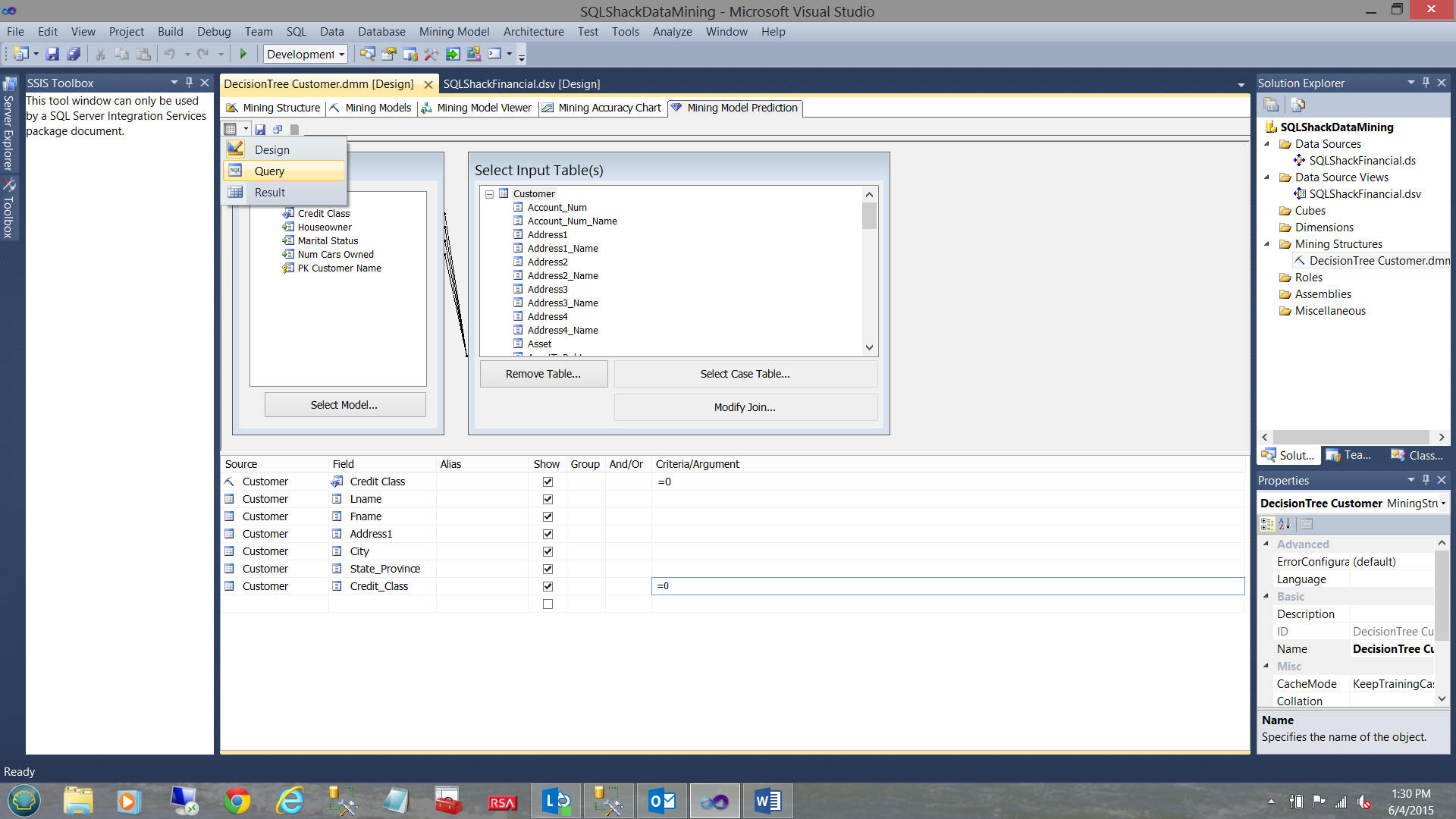
Selecting the query option shown in the screen dump above, we select “Query”.
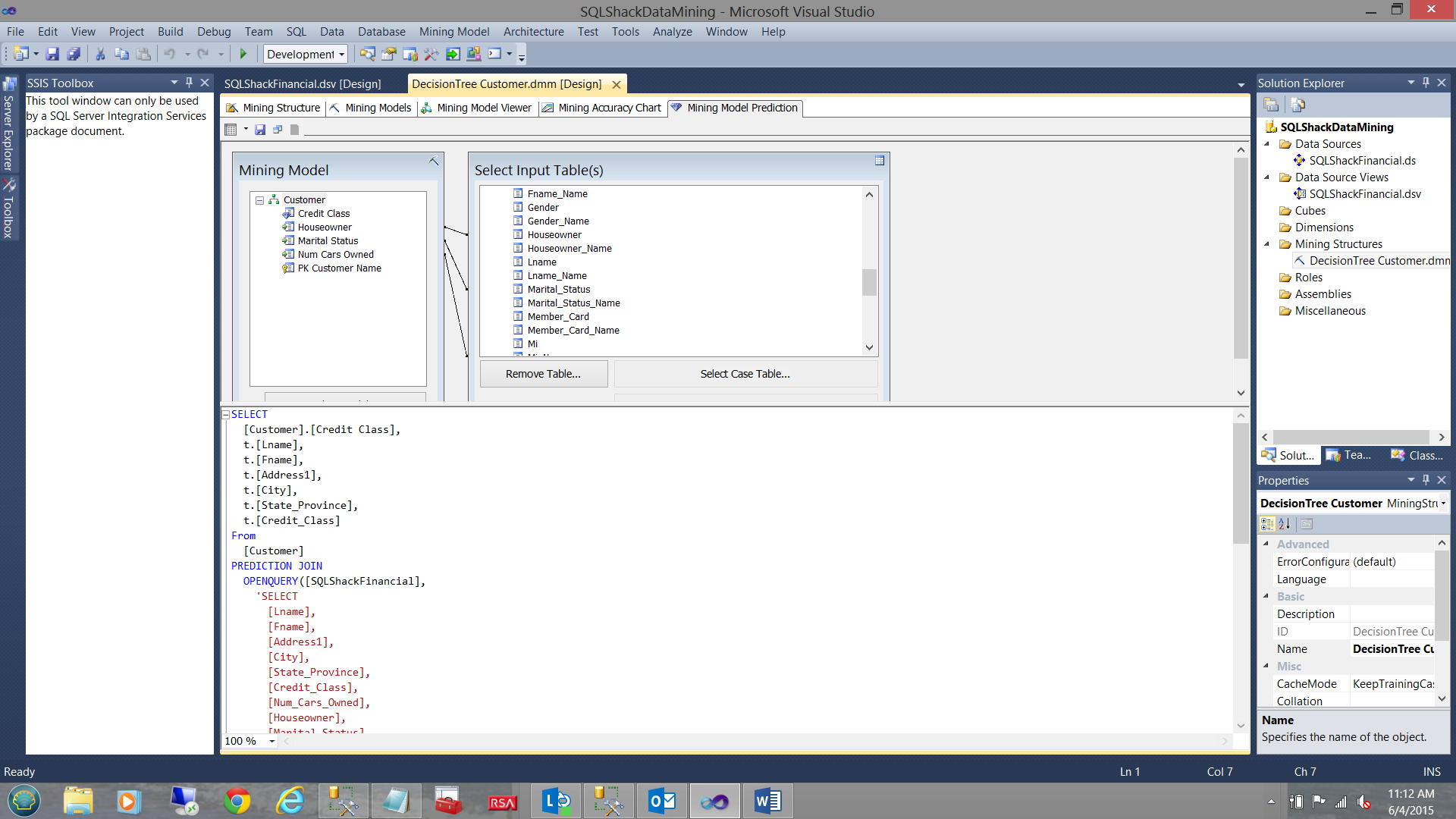
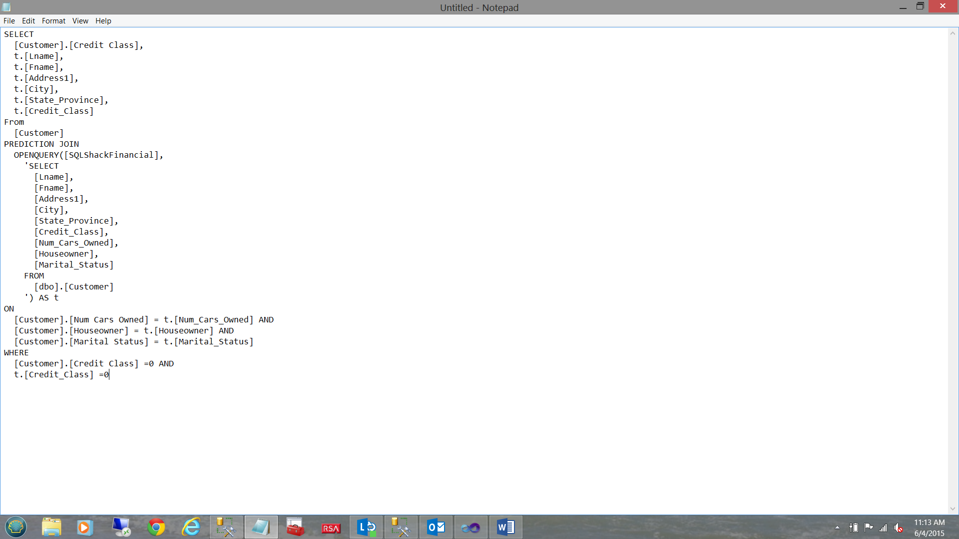
The DMX (Data Mining Expression) used to produce the results (that we just saw) is displayed.
|
1 2 3 4 5 6 7 8 9 10 11 12 13 14 15 16 17 18 19 20 21 22 23 24 25 26 27 28 29 30 31 32 33 |
SELECT [Customer].[Credit Class], t.[Lname], t.[Fname], t.[Address1], t.[City], t.[State_Province], t.[Credit_Class] From [Customer] PREDICTION JOIN OPENQUERY([SQLShackFinancial], 'SELECT [Lname], [Fname], [Address1], [City], [State_Province], [Credit_Class], [Num_Cars_Owned], [Houseowner], [Marital_Status] FROM [dbo].[Customer] ') AS t ON [Customer].[Num Cars Owned] = t.[Num_Cars_Owned] AND [Customer].[Houseowner] = t.[Houseowner] AND [Customer].[Marital Status] = t.[Marital_Status] WHERE [Customer].[Credit Class] =0 AND t.[Credit_Class] =0 |
This is our jumping off point for today’s discussion.
Turning our DMX data into valuable information
Our first task is to address the most efficient and effective manner to create queries that may be utilized for reporting purposes.
Most of us know the trials and tribulations of filtering data from MDX expressions. Somehow it is a nightmare. DMX queries are no easier nor as versatile nor as flexible as T-SQL.
We are going to attack our problem by utilizing the “Hamburger” method (see below).
 |
T-SQL Select statement |
| DMX | |
| T-SQL predicate |
Our first task is to create a linked server through to our Data Mining Analysis database.
Our database is shown in the screenshot above.
The code to create the linked server (linking our relational database “SQLShackFinancial” on Server STEVETOPMULTI to the database “SQLShackDataMining” on the analysis server STEVETOPMULTI) is shown below:
|
1 2 3 4 5 6 7 8 9 10 11 12 |
USE master GO EXEC sp_addlinkedserver @server='SQLShackDataMining', -- local SQL name given to the linked server @srvproduct='', -- not used @provider='MSOLAP', -- OLE DB provider @datasrc='R9-WXL90\STEVETOPMulti', -- analysis server name (machine name) @catalog='SQLShackDataMining' -- default catalog/database |
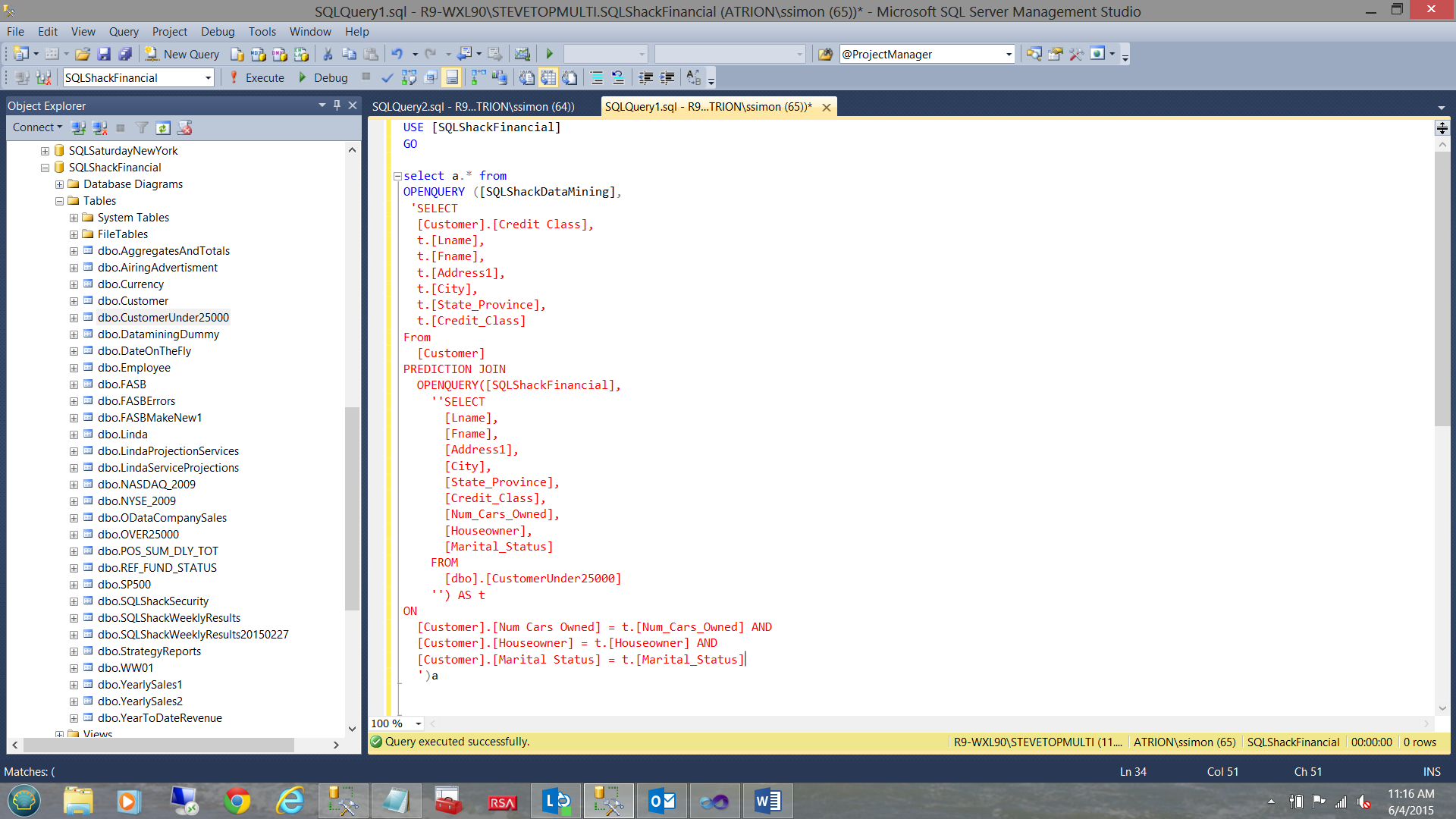
The screenshot above shows us the DMX code that we shall be using. This code is the “meat portion of the burger”.
We change the code slightly as may be seen in the screenshot below:
And the result set of this simple query may be seen in the screen dump below:
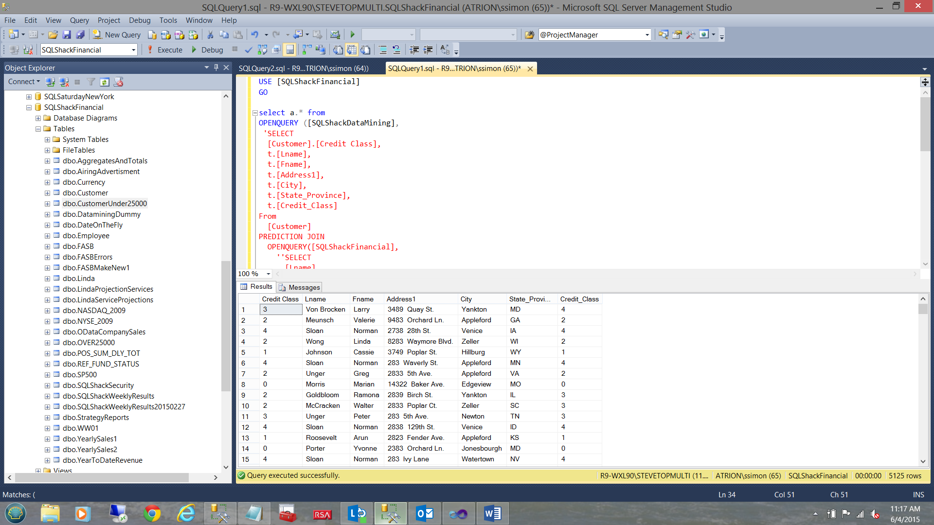
The code for our query may be found in Addenda 1.
Let us get busy with the fancy leg work
As described in the introduction, we wish to utilize our data mining “data” and to turn it into valuable information. This said let us take advantage of the “Hamburger” approach and modify our crude query to make reporting simpler and more effective.
By inserting the contents of the query (that we just ran into a table written to disk), we can see the field names as SQL Server Management Studio knows them (see below).
|
1 2 3 4 5 6 7 8 9 10 11 12 13 14 15 16 17 18 19 20 21 22 |
USE [SQLShackFinancial] GO /****** Object: Table [dbo].[DataminingDummy] Script Date: 6/3/2015 1:03:53 PM ******/ SET ANSI_NULLS ON GO SET QUOTED_IDENTIFIER ON GO CREATE TABLE [dbo].[DataminingDummy]( [Credit Class] [bigint] NULL, [Lname] [ntext] NULL, [Fname] [ntext] NULL, [Address1] [ntext] NULL, [City] [ntext] NULL, [State_Province] [ntext] NULL, [Credit_Class] [smallint] NULL ) ON [PRIMARY] TEXTIMAGE_ON [PRIMARY] GO |
We can now modify our query accordingly
We can even remove the DMX predicate all together and let the report query define the final predicate.

Further, we can create very dynamic predicates which may accept parameter (see below).
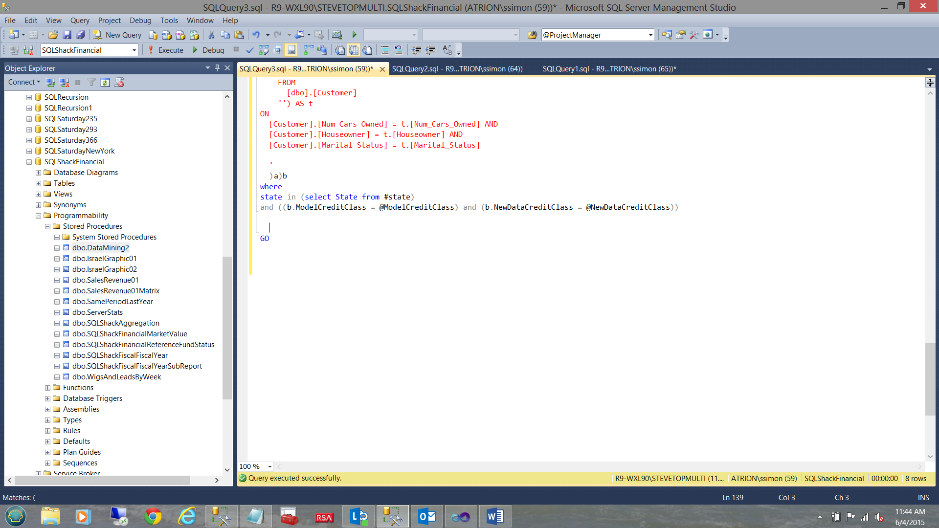
More on this topic in a few minutes after we construct our first report.
Reporting from our mining model
Opening SQL Server Data Tools, we create a new Reporting Services Project. Should you not be familiar with the process, please do see one of my earlier articles on SQLShack.com where the process is described in detail.
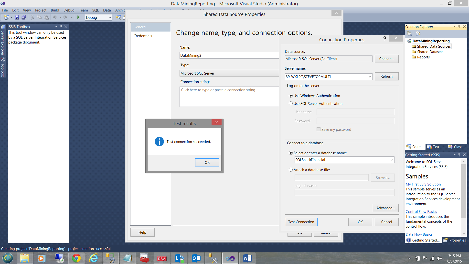
As always, we create a new Data Source to the “SQLShackFinancial” database (see above).
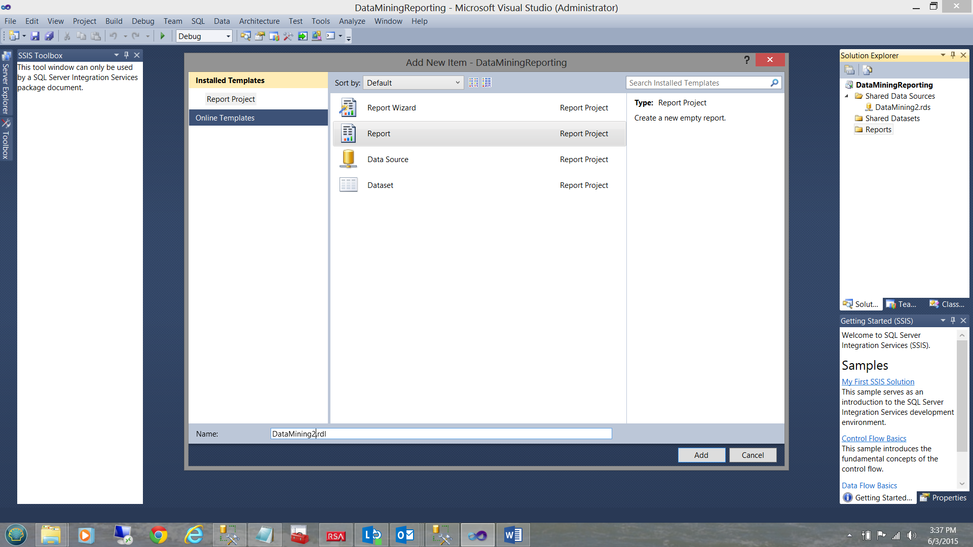
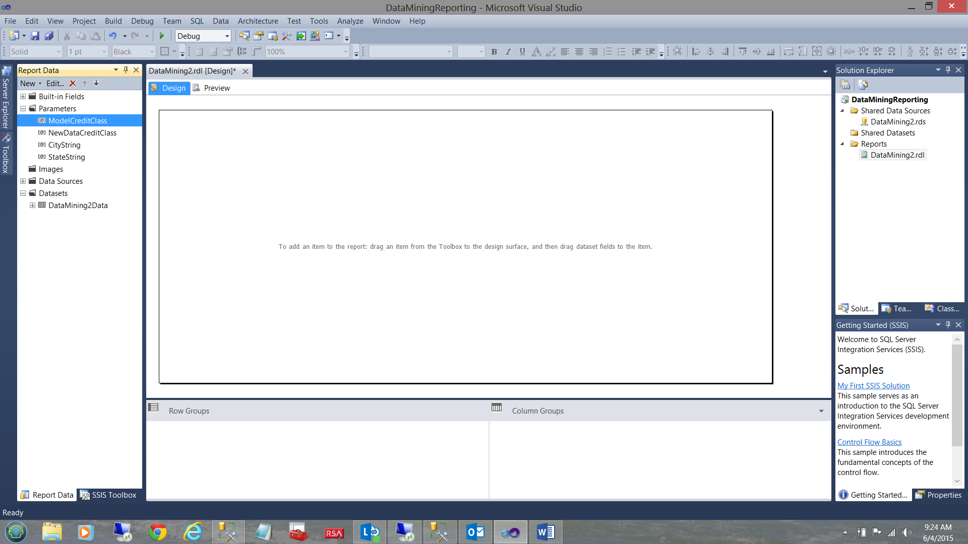
We add a new report and name it DataMining2 (see above).
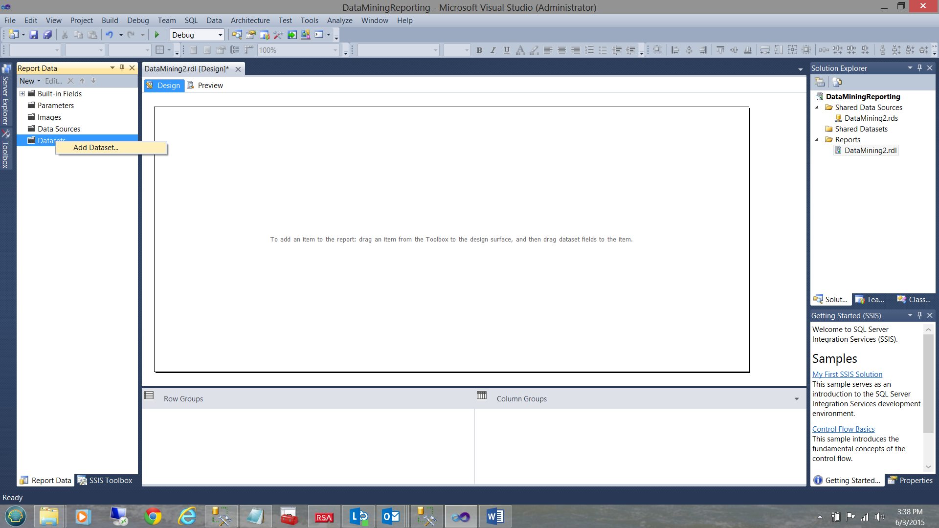
As always, our next task is to create a dataset (see above).
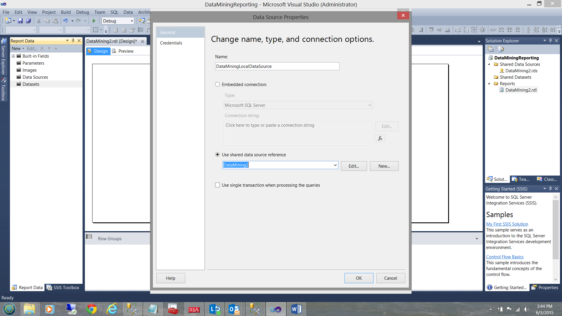
First we create a local data source which references our shared data source”DataMining2”.
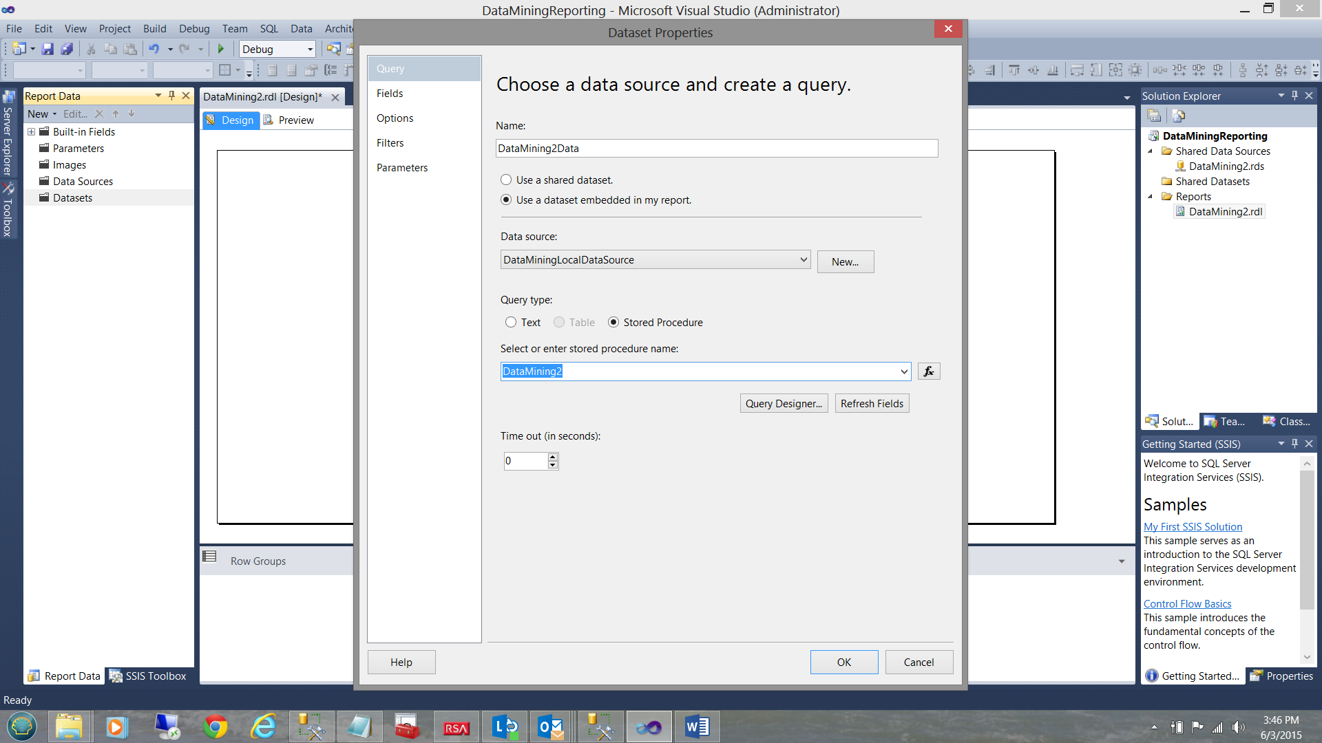
We set the data source to point to our stored procedure DataMining2 (which was created with the code that we just discussed). See the code listing in Addenda 2.
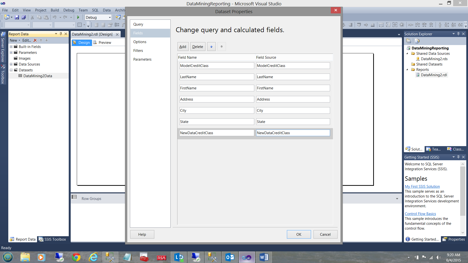
By clicking on the fields tab (see above), we note all the fields from the stored procedure, “DataMining2”. We click “OK” to leave the “Dataset Properties” dialog box.
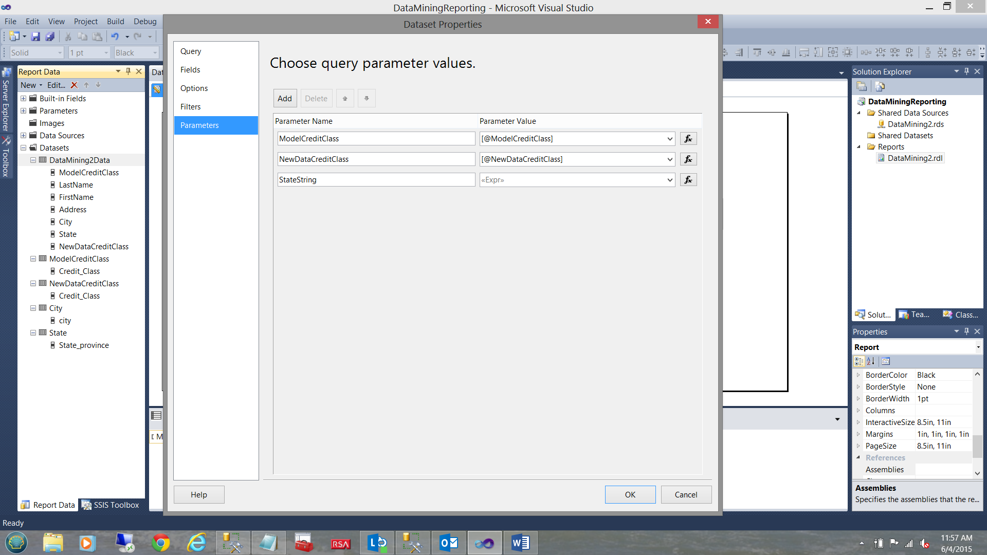
We are in now in the position to add a few parameters to our report.
The astute reader will note that these parameters have been added to the Parameters Tab due to the fact that Reporting Services has noted that the stored procedure requires three parameters.
Creating the dataset which will supply the parameter values for the “ModelCreditClass” parameter.
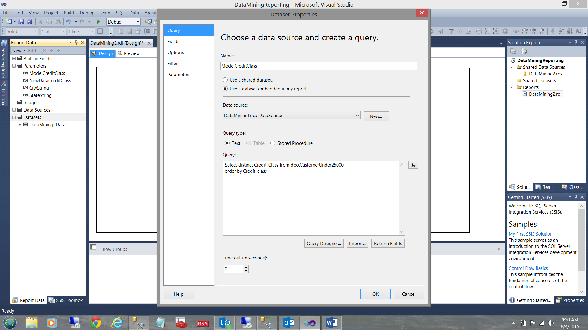
In a similar manner to which we created the DataMining2Data dataset, we create a “ModelCreditClass” dataset (see above). Note that the data that we require may be obtained by utilizing a simple SQL Statement.
|
1 2 3 |
Select distinct Credit_Class from dbo.CustomerUnder25000 order by Credit_class |
In a similar manner, we create another dataset for “NewDataCreditClass”. As a reminder to the reader, “NewDataCreditClass” is the credit class that was assigned by a credit rating firm (within the new/ fresh data). This way we are able to validate our prediction with values from a professional firm.
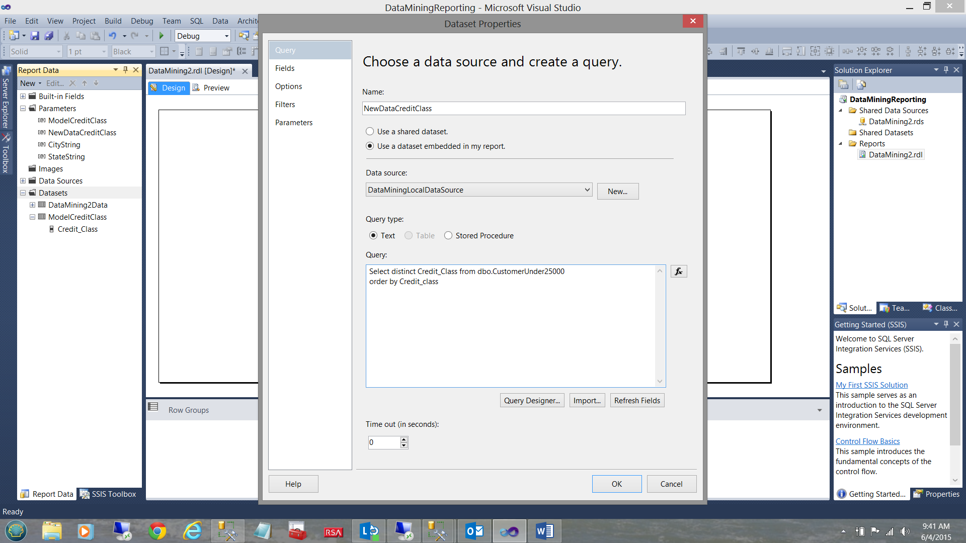
Once again, the astute reader will note that we use the same SQL query to populate this dataset and the numbers are same as the source of the number data is not really relevant.
Moving back to the “Parameter” tab, we double click the “ModelCreditClass” parameter.
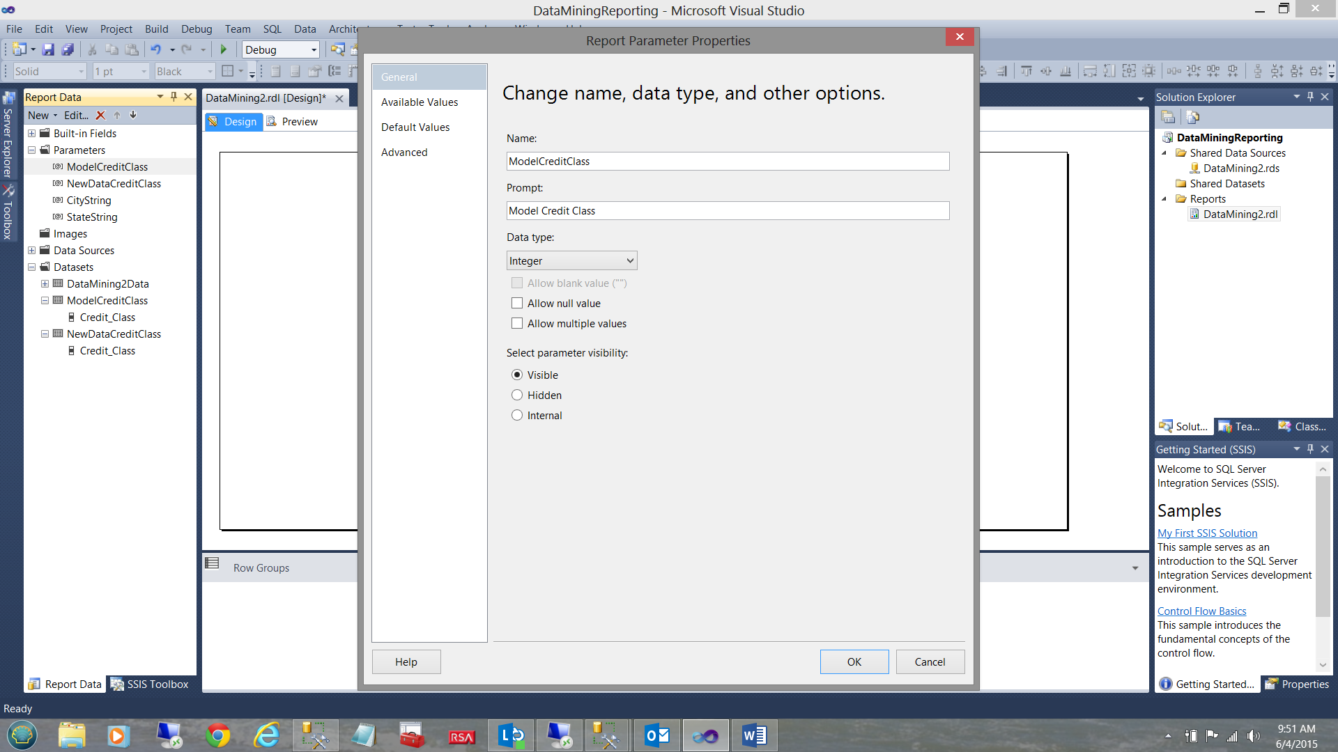
The “Report Parameter Properties” dialog box opens (see above).
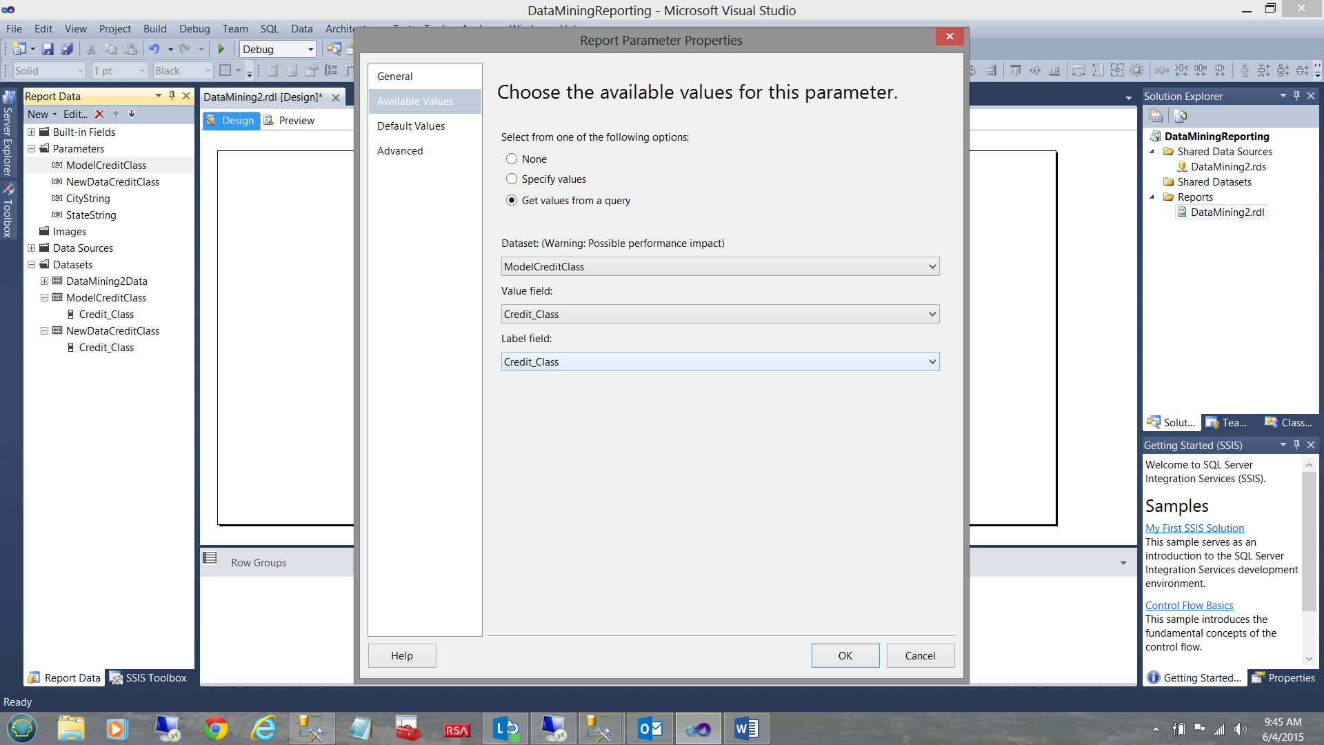
On the “Available Values” tab, we click the “Get Values from a query” box and set the “Dataset” to the “ModelCreditClass” dataset that we just created.
Finally, we set the “Value” and “Label Fields” to “Credit_Class”. We then click “OK” to exit the dialogue box.
In a similar fashion we do the same tasks to provide the “NewDataCreditClass” parameter with values (see below).

Working with the “State” parameter
We are going to handle the “State” parameter in a different fashion. We are going to initialize the parameter as a multi-select parameter. Before continuing with the configuration of this parameter, we must once again create a dataset.
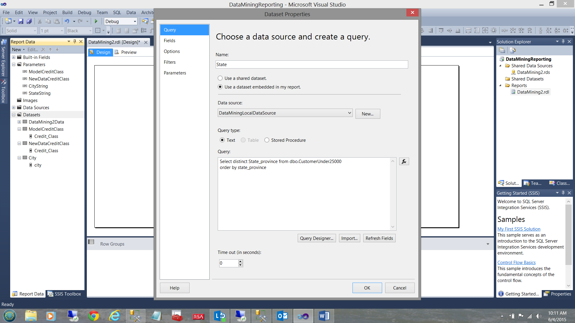
The “State_Province” dataset is shown above and is configured as we have configured the other datasets discussed above.
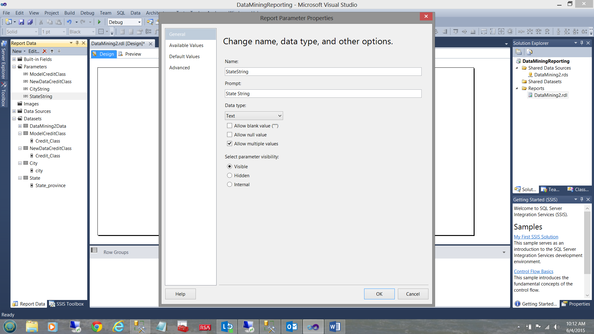
The setup of the “StateString” is similar to the other parameters described above. The only difference is that we check the “Allow multiple values” checkbox (see above).
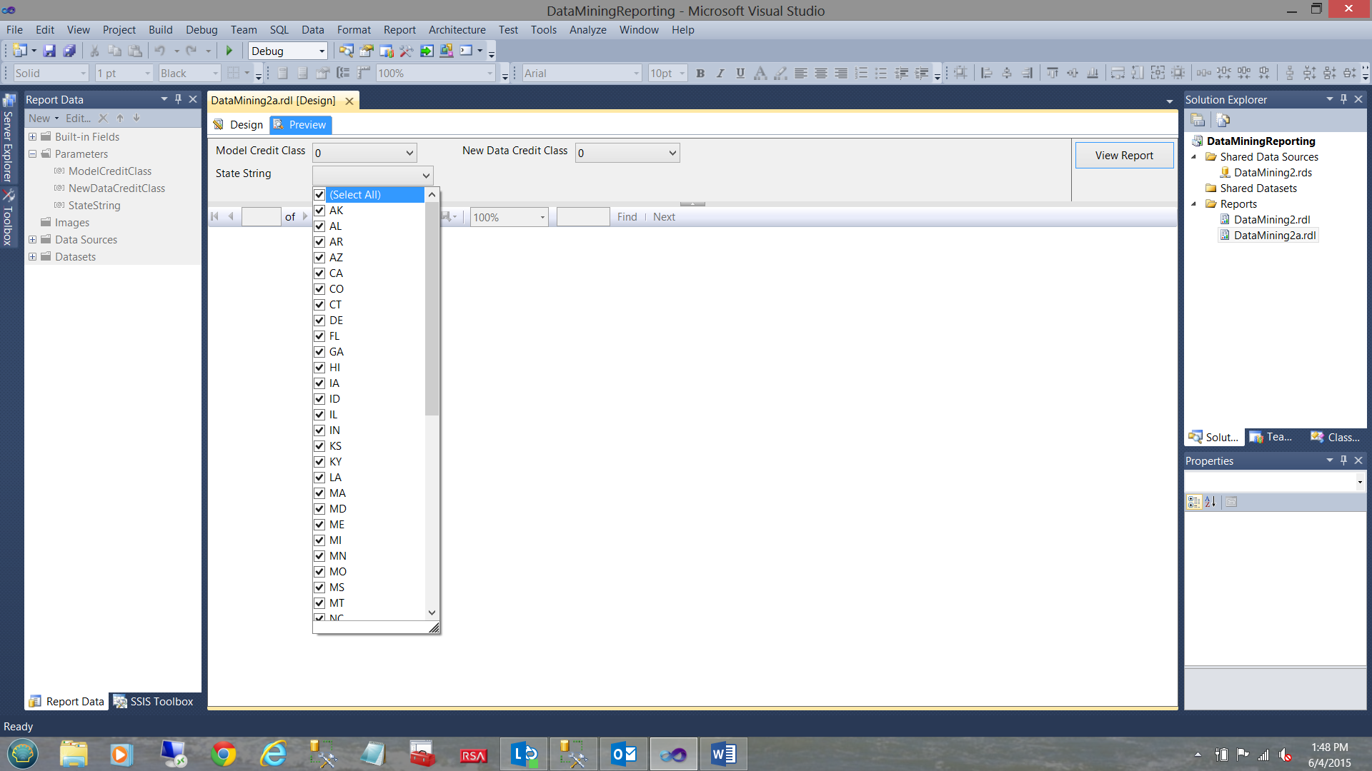
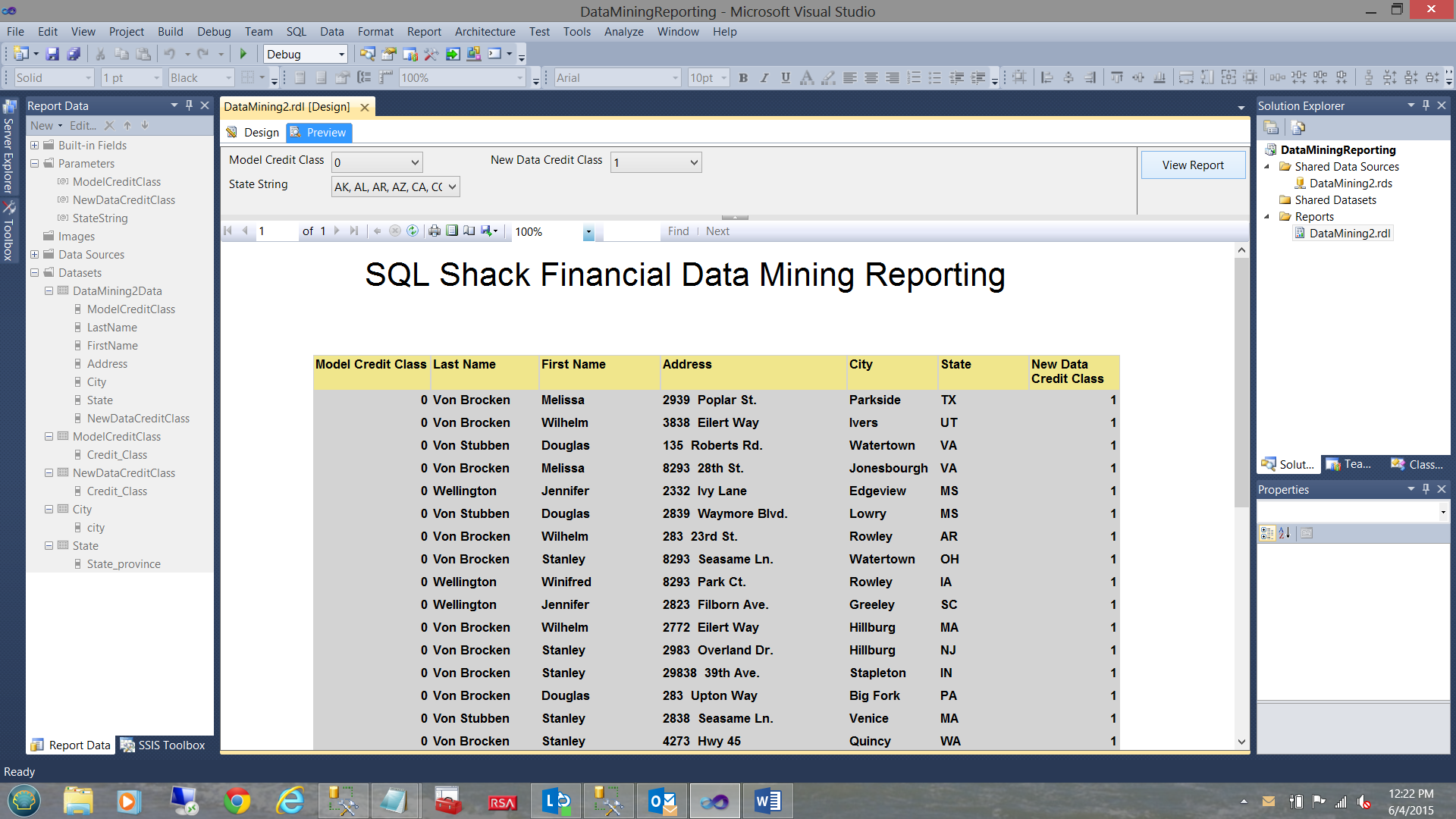
Having a preview of what we have created thus far, we click on the “Preview” tab. The report appears as shown above.
Our last and most important task is to configure the “DataMining2Data” dataset to handle multiple values for the “State”.
Configuring the State Parameter
Why are we required to configure the remaining parameter in a special manner? The answer is simply that as we have opted to pass MULTIPLE states to the stored procedure. This being the case, we must “tell” the parameter to keep concatenating the values that we select AND then to pass those concatenated values onto the stored procedure. We shall discuss how the stored procedure handles that whopping big string in just a few moments, but let us not get ahead of ourselves.
Opening the “DataMining2Data” dataset, we click on the “Parameters” tab (see above). We note that there is a “table” like configuration box with which we shall now work. For the “StateString” parameter, we click on the function button immediately to the right of the “Parameter Value” cell.
The “Expression” dialogue box opens.
We change the value “ =Parameters!StateString.values” to =JOIN(Parameters!StateString.Value,”,”)
See below:
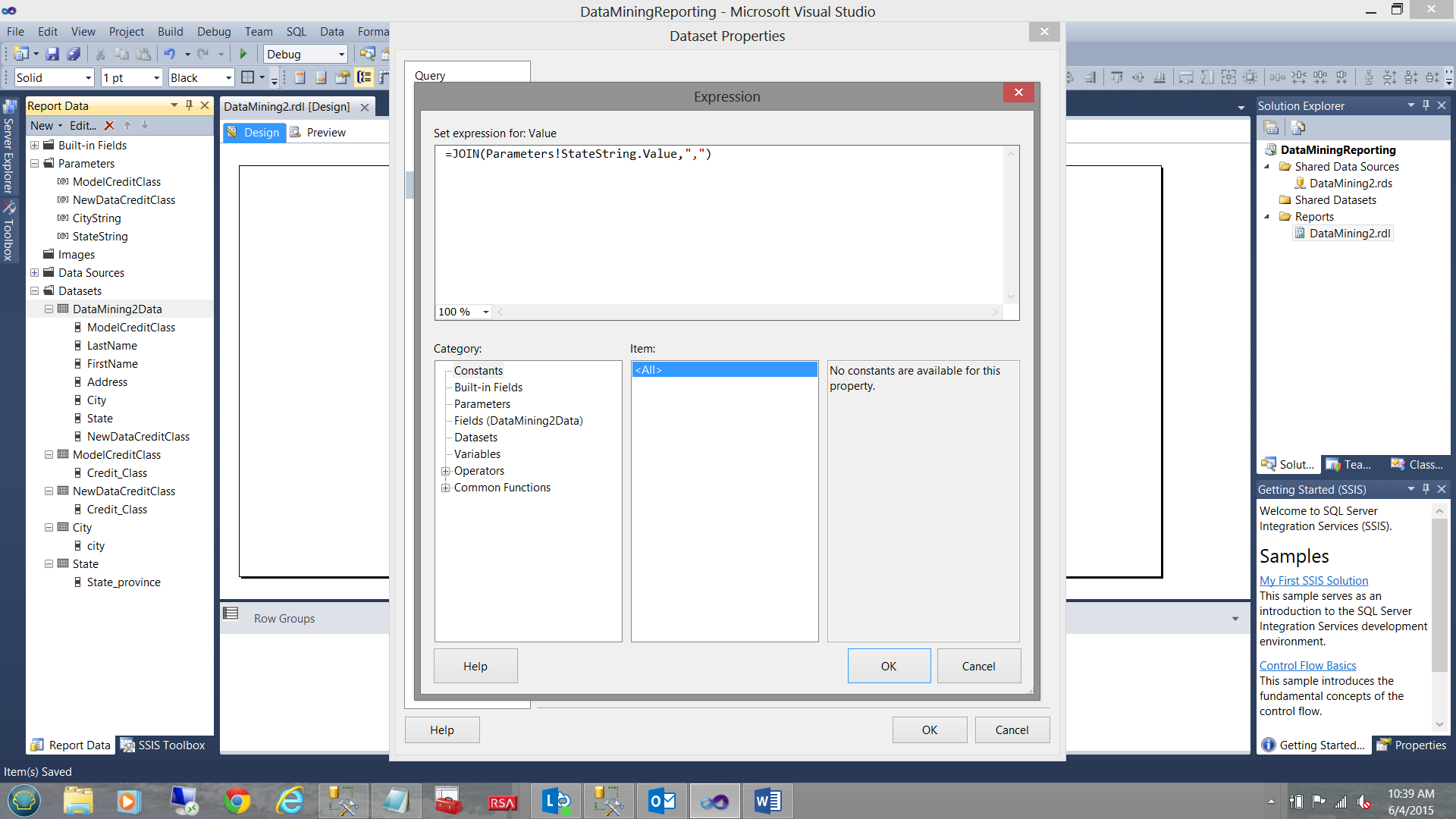
We click “OK” and the “Expressions” dialog box closes.
The Report Body
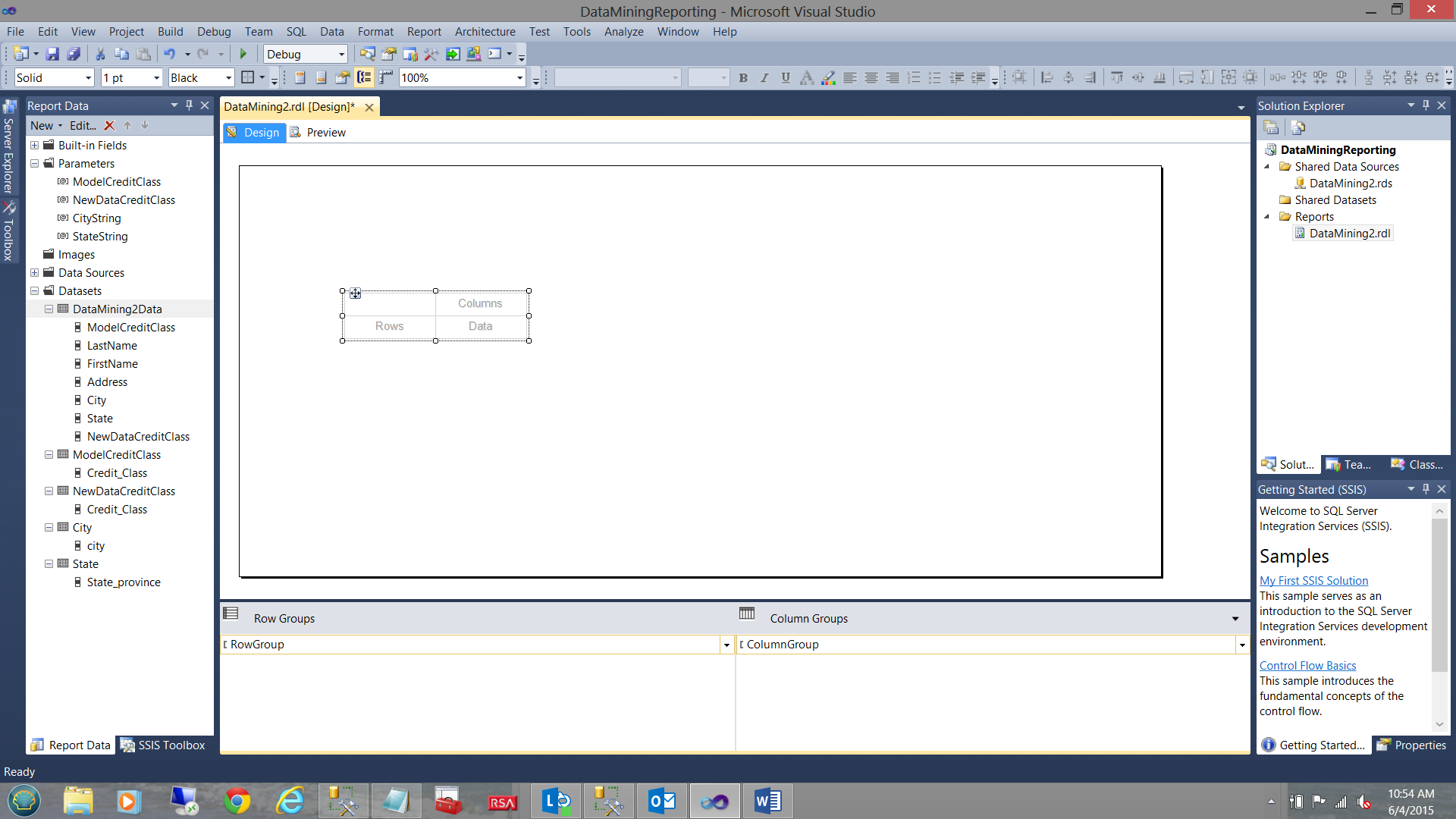
Now that our infrastructure is complete, we are now in a position to design our report body. We begin by dragging and placing a “Matrix” (from the toolbox) onto the work surface (see below).
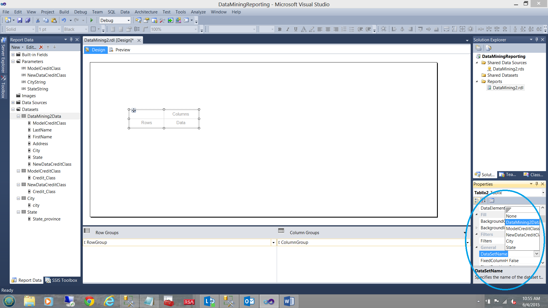
Our next task is to link the matrix to the dataset “DataMining2Data” (see below).

Our first task is to right click on the “Column Groups” tab (see above) and to “Delete” the group only.
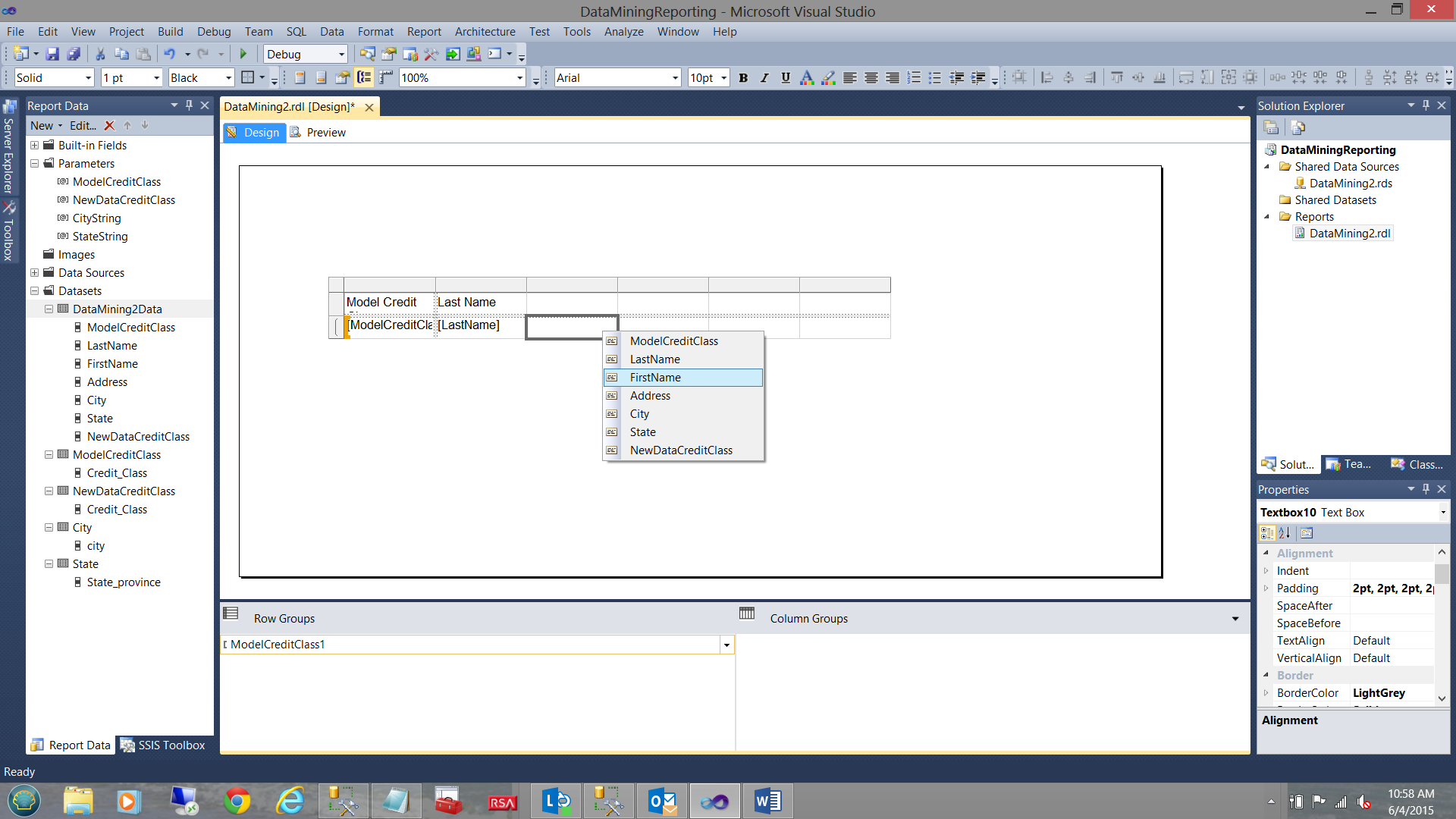
We then add a few more columns to our matrix and place our dataset fields into the matrix, one by one (see above).
We are now in a position to configure the row grouping and as we are interested in viewing all rows in a non-aggregated state, then we must group by several fields. We double click the “ModelCreditClass1” Row Grouping.
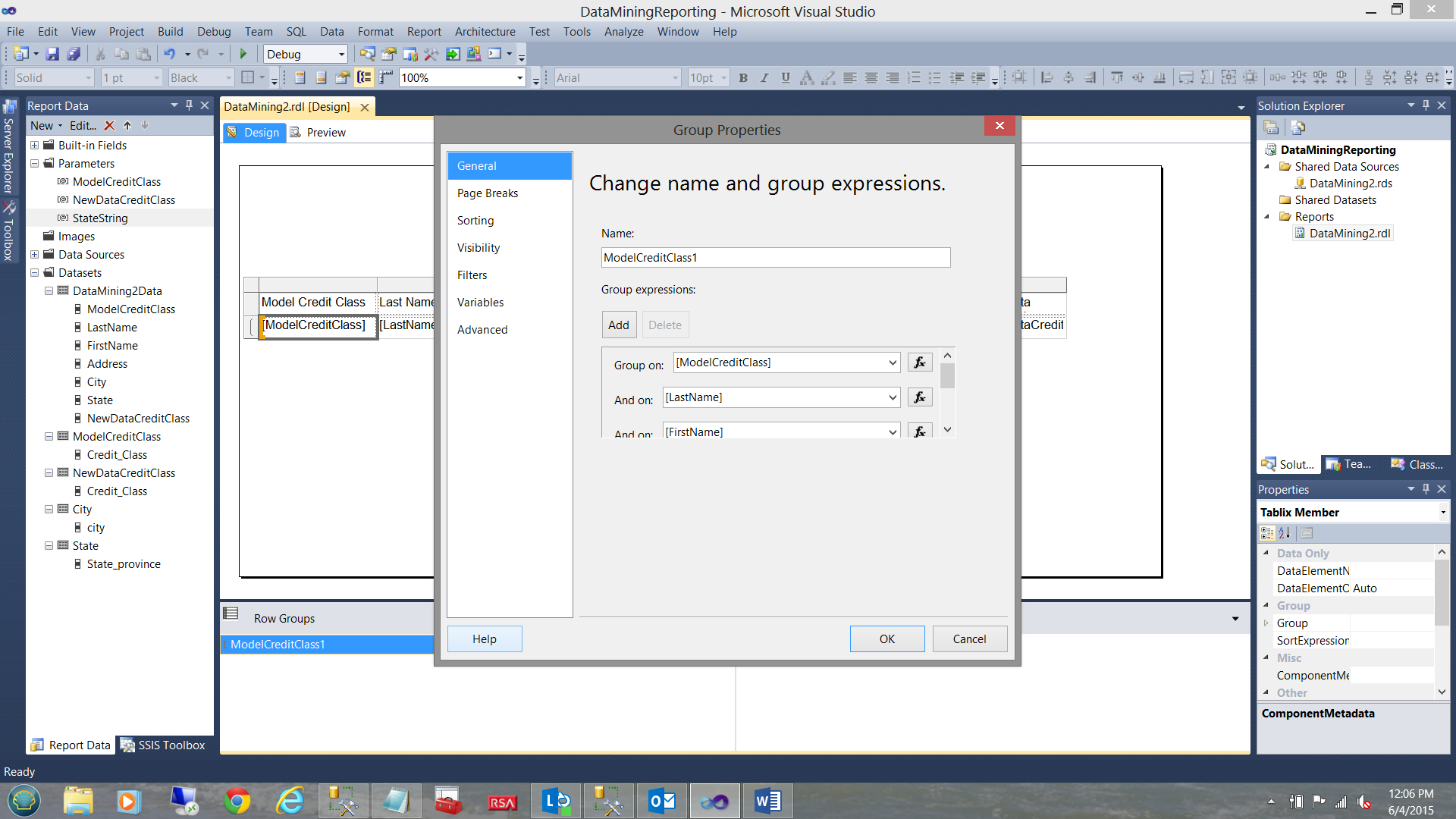
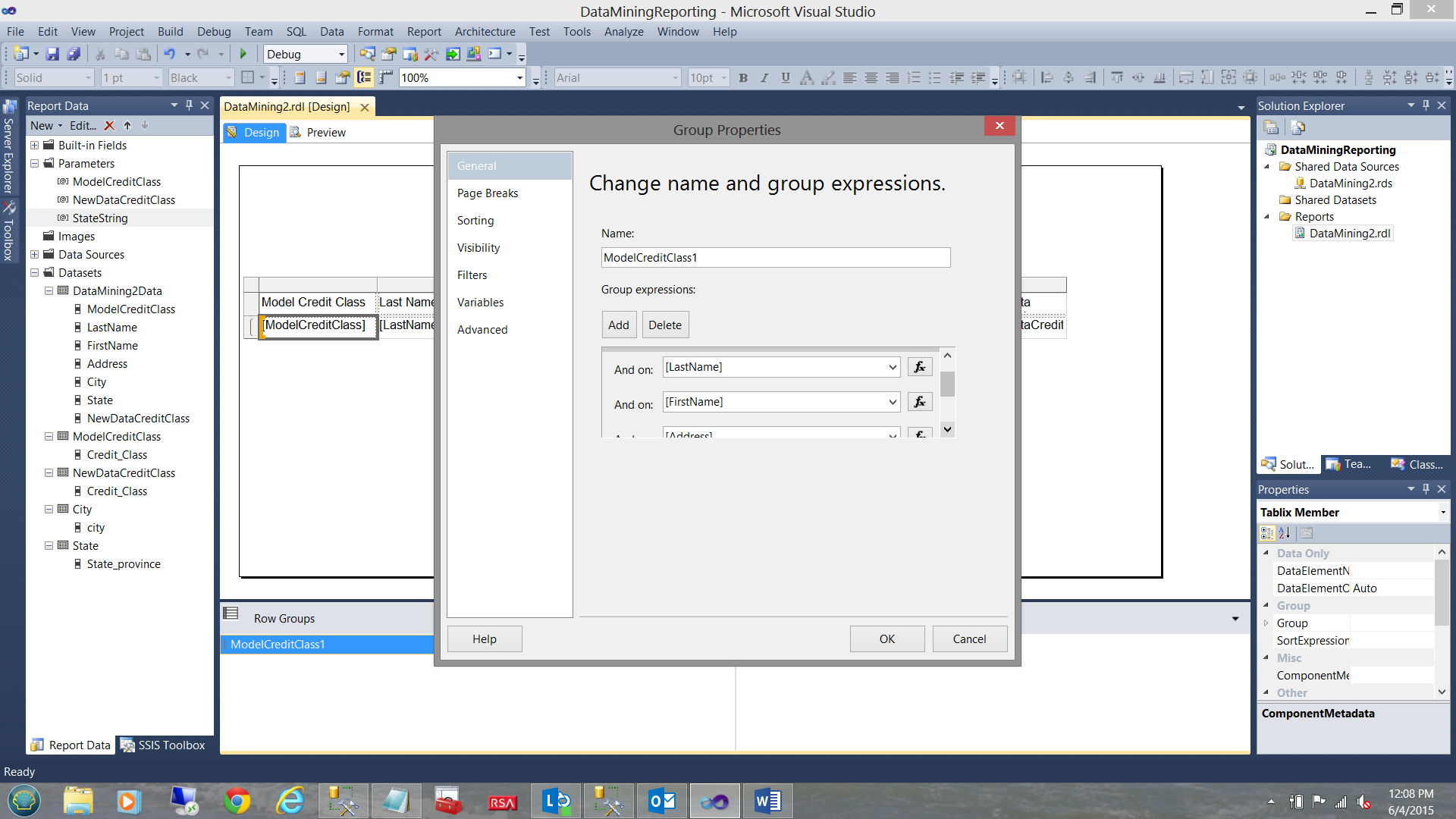
The “Group Properties” Dialog box opens. We add the following groupings by clicking on the Add button (see below). These grouping fields include “ModelClassCredit”, “LastName”, “FirstName”, Address, City, and State.
We click OK to leave the “Group Properties” dialogue box and find ourselves back on our work surface (see below).
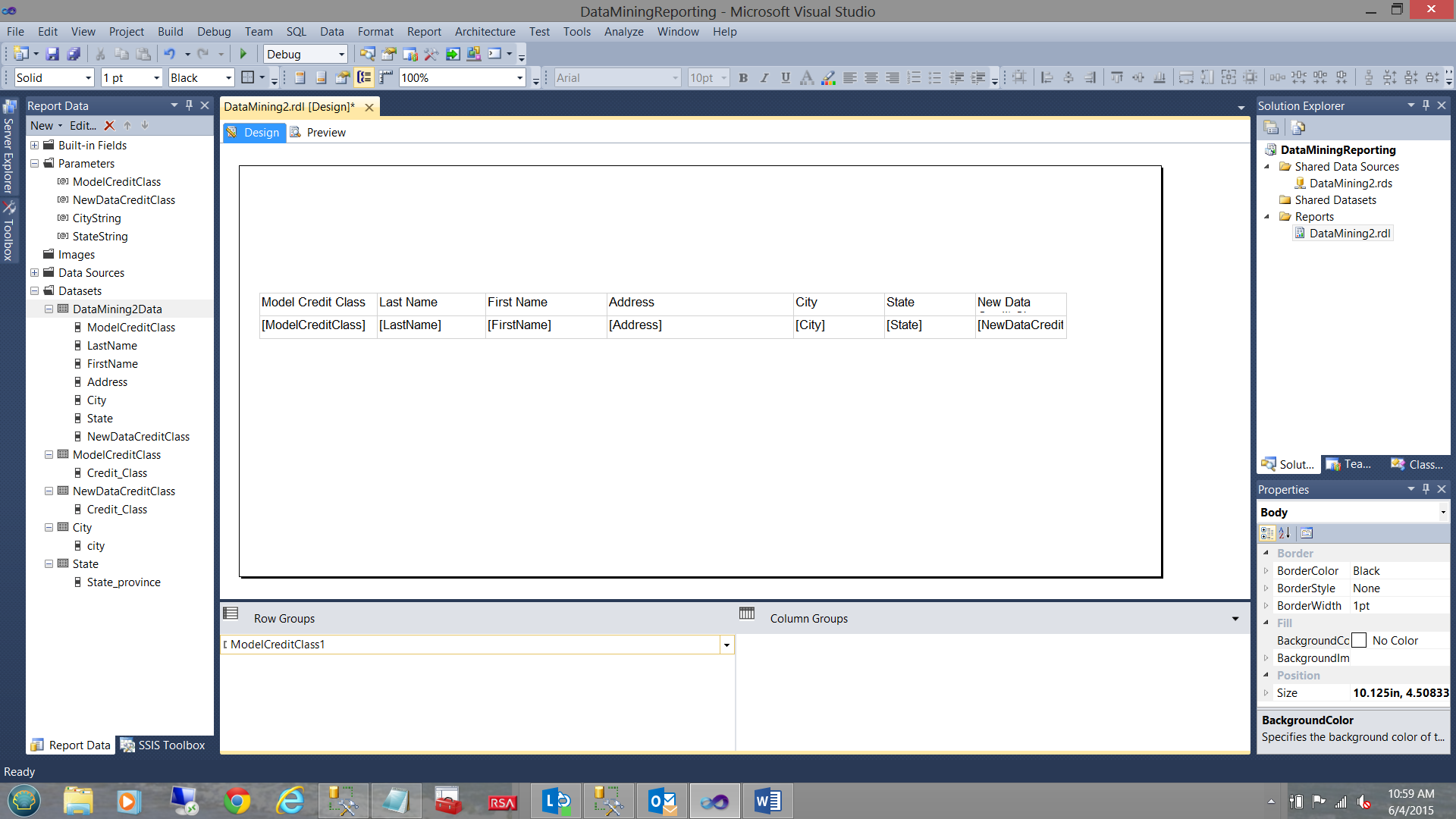
Our completed matrix may be seen above.
Tidying up a tad
We first add a bit of color to our Matrix (see below).
The one issue that most of us hate it when scrolling down on a report that the column headers tend to disappear. Let us changes to the header properties to scroll down with us, PLUS have them visible on each report page.
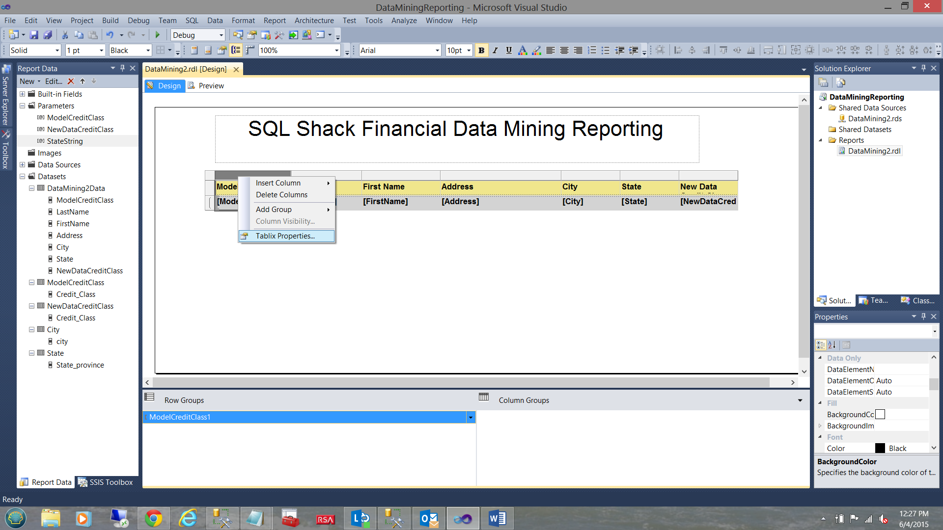
We right-click upon the Column Header as shown above within the grey box and bring up the “Tablix Properties” dialogue box.
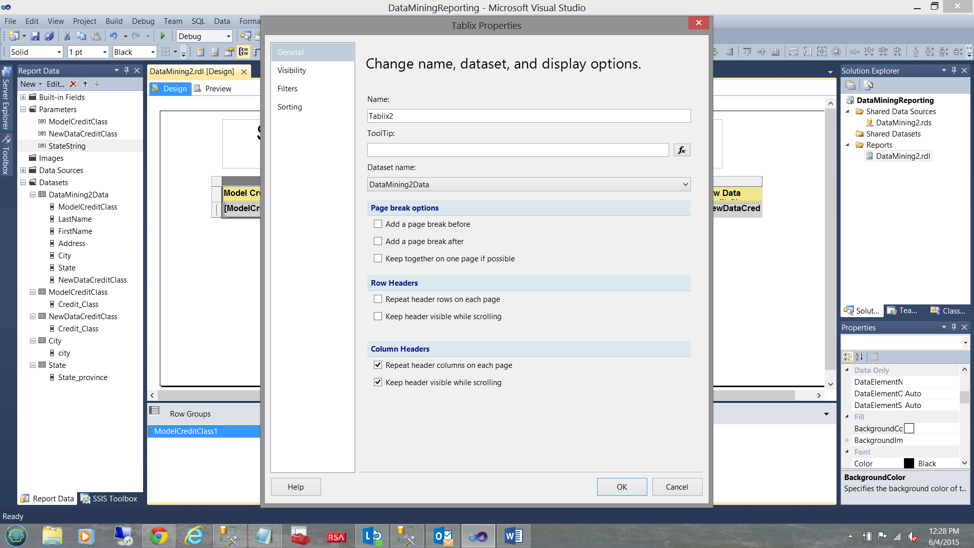
We then “check” the “Repeat Header columns on each page” and the “Keep header visible while scrolling” option within the “Column Header” dialogue box (see above). We then click “OK” to leave the “Tablix Properties” dialogue box.

We note that the column headers are STILL visible as we approach the bottom of the page (see above).
Conclusions
We have once again come to the end of another get-together. In this session we have looked at the constructive utilization of the “mined” data, turning it into valuable information.
We saw the DMX code that is generated by the model based upon our business rules and we were introduced to the “Hamburger” approach to data extraction. This approach permitted us to mine the data and yet utilize standard T-SQL to define the predicate and re-format the data. Through using the code in Addenda3 we are able to strip the long selection of state names and place the respective values into a temporary table to be utilized by our report predicate.
As always, should you have any questions or concerns, please feel free to contact me.
In the interim, happy programming!
Steve has presented papers at 8 PASS Summits and one at PASS Europe 2009 and 2010. He has recently presented a Master Data Services presentation at the PASS Amsterdam Rally.
Steve has presented 5 papers at the Information Builders' Summits. He is a PASS regional mentor.
View all posts by Steve Simon
- Reporting in SQL Server – Using calculated Expressions within reports - December 19, 2016
- How to use Expressions within SQL Server Reporting Services to create efficient reports - December 9, 2016
- How to use SQL Server Data Quality Services to ensure the correct aggregation of data - November 9, 2016