

The Multidimensional Cube option of Analysis Services has handled many-to-many relationships with ease for many versions before 2016. The Tabular had a work around using DAX formulas until the release of SQL Server 2016. There are still some limitations to many-to many in Tabular but of course, there are some “tricks” to overcome the limitations. But, the many-to-many relationship will be in businesses data for many years to come. A solution has to be provided when it comes to Analysis Service databases.
Before going to the development and support of many-to-many in Analysis Services, the ETL of a reporting application has to format the data in tables conducive to supporting this option. This might be referred to as a bridge table. The data in the transaction table is “bridged” to the many possible supporting categories. The Adventure Works DW data provides a great example with many Sales Reasons related to many Internet Sales Line Items.
Figure 1 shows an example of the design of these tables.
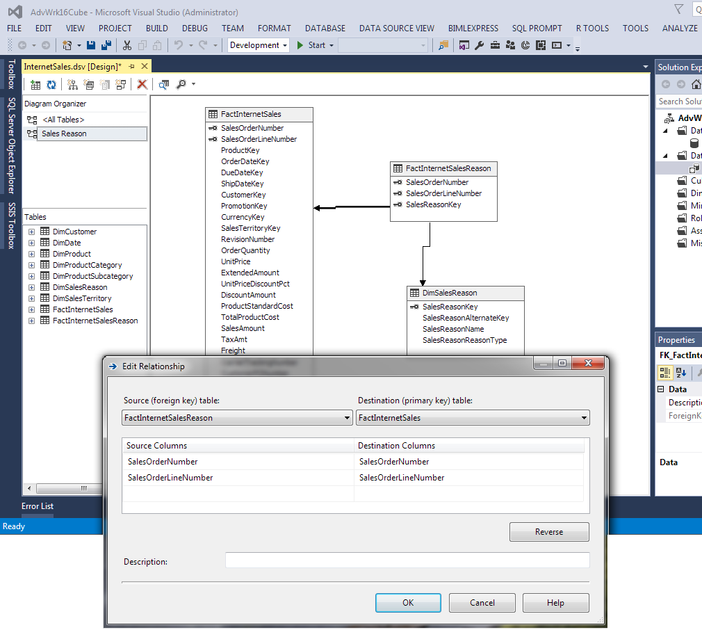
The Edit Relationship in Figure 1 shows in a cube the relationship between 2 tables with multiple columns – SalesOrderNumber (Order Number) and SaleOrderLineNumber (Order Line Number). This bridge table, FactInternetSalesReason, bridges the Sales Reasons from the DimSalesReason dimension table to the FactinternetSales fact table by these 2 columns. The FactInternetSalesReason table can have multiple entries for the same Order Number plus Order Line Number. The example in the table below shows 2 different Sales Order Number with 3 different Sales Reason.
| SalesOrderNumber | SalesReasonName |
| SO51214 | On Promotion |
| SO51214 | Other |
| SO51214 | Price |
| SO51298 | On Promotion |
| SO51298 | Other |
| SO51298 | Price |
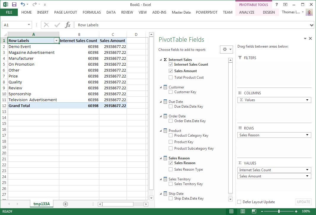
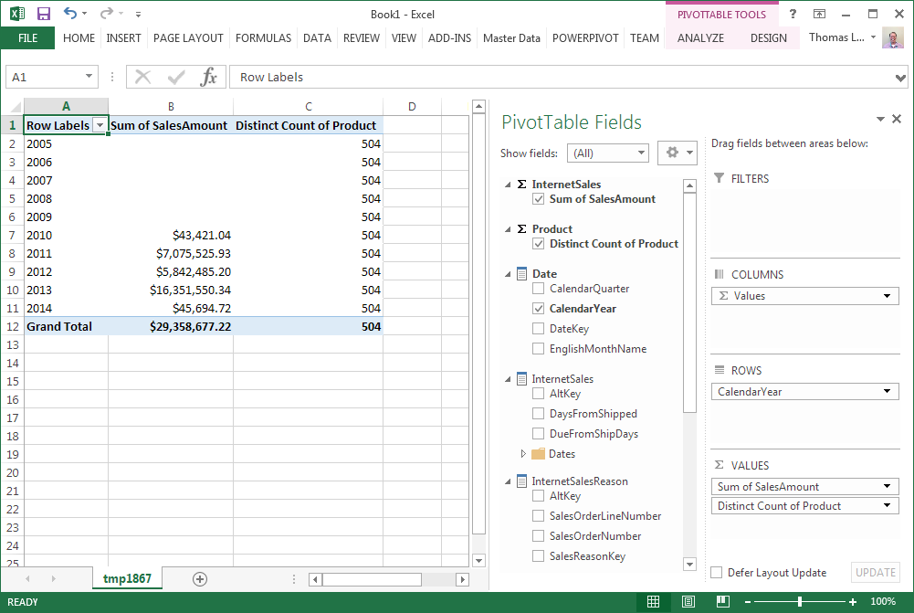
Figure 2 shows the Analyze in Excel when there is no relationship between Sales Reason and Internet Sales for the cube. This is the same output initially received with Tabular as well. Many-to-many relationships are not automatically assigned with building a cube or tabular model through the wizards. There is more work to be done after the wizard completes. The Sales Count and Sale Amount measures are summed on all rows rather than the Sales Reason slicer used in Figure 2.
The relationship is not a regular relationship for the Dimension Relationship in the Cube. But before setting the relationship, the Sales Reason (DimSalesReason table) and Fact Internet Sales (FactInternetSales table) dimensions need to be created plus a Measure Group for fact table FactInternetSalesReason. The measure can be a count of rows and hidden through the Visible property of the measure. Once these are created, the many-to-many relationship can be created in the Cube Dimension Relationship between the Sales Reason Dimension and Internet Sales Measure group like in Figure 3.
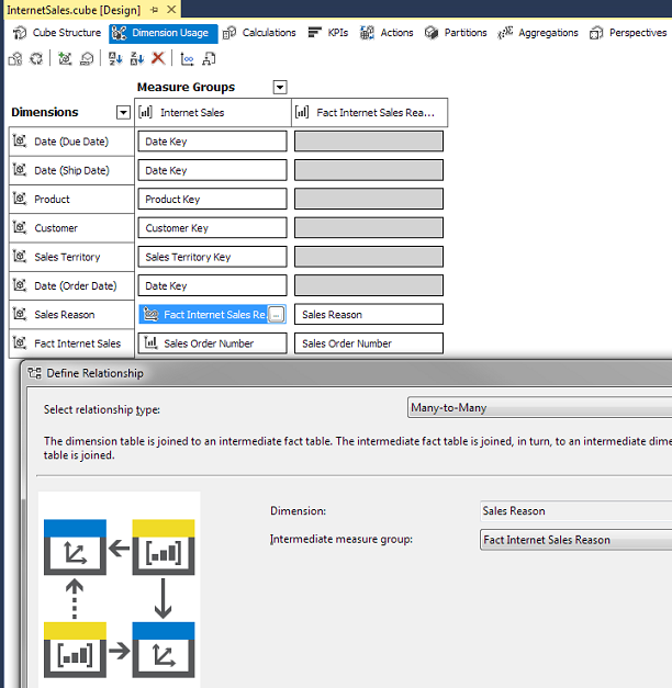
Below the Sales Reason relationship to Internet Sales measure group is a Fact Relationship between Fact Internet Sales dimension and Internet Sales measure group. Fact tables can be dimensions in Analysis Service and contain attributes like PO Number or Freight Company. It can also be created for this relationship and made Visible = False in the cube. The Sales Reason and Fact Internet Sales dimensions are related to new measure group by regular relationships.
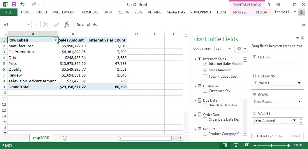
Figure 4 now shows correct counts and dollar amounts while Analyzing in Excel. The Sales Amount total as Grand Total is the correct total of all sales filtered. But the Sum of the Sales Reason totals in the pivot table will be more than the grand total because of sales having multiple sales reasons. Training end users about this variation are important.
The Tabular Model of Analysis Services uses a new feature in SQL Server 2016 called bi-directional filtering. Bi-directional filtering is used for many-to-many. The creation of bi-directional filtering is for filtering through one table, say a fact table, to an aggregation in a dimension table. Some might go activate this on every relationship, but Microsoft warns not to do this. Just implement where needed.
The only many-to-many this will work with is a 3 table many-to-many. Figure 5 shows the Fact Internet Sales, Fact Internet Sales Reason and Sales Reason in a Tabular Model. Do not use this when more than 3 tables are involved in a many-to-many relationship.
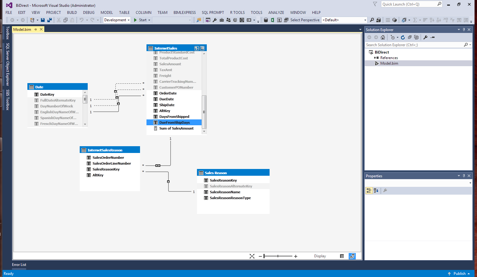
What cannot be seen in this example is the columns used to relate InternetSalesReason to InternetSales. The relationships in the Tabular Model (and in Power BI) can only be one column. So, this example uses a calculated column in the InternetSales and InternetSalesReason table. Figure 6 shows this relationship.
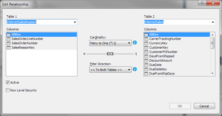
Also, the Filter Direction drop-down shows “To Both Table” instead of to the many sides of a relationship. This is the bi-directional filtering option. The column used to relate the 2 tables is called AltKey. Figure 7 shows the calculated column in the InternetSalesReason table.
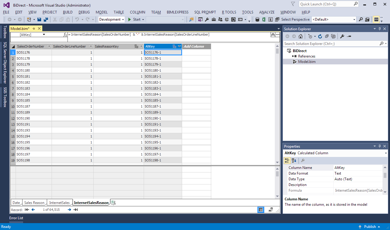
The AltKey computed column uses this logic –InternetSalesReason [SalesOrderNumber] & “-” & InternetSalesReason [SalesOrderLineNumber]. The SalesOrderNumber is concatenated with the SalesOrderLineNumber with a dash between the 2 values. This column creates an alternate key for the tables. Since it is created in both InternetSales and InternetSalesReason, they can be used to join the 2 fact tables. Remember, the InternetSalesReason table is the bridge table between DimSalesReason and FactInternetSales.
The Bi-Directional filtering can be used in another way. Says the end user wants to view a count of distinct products associated with the Sales list by a particular year. A normal many-to-one relationship will not be able to show that. Figure 8 shows the normal DimProduct relationship to InternetSales.
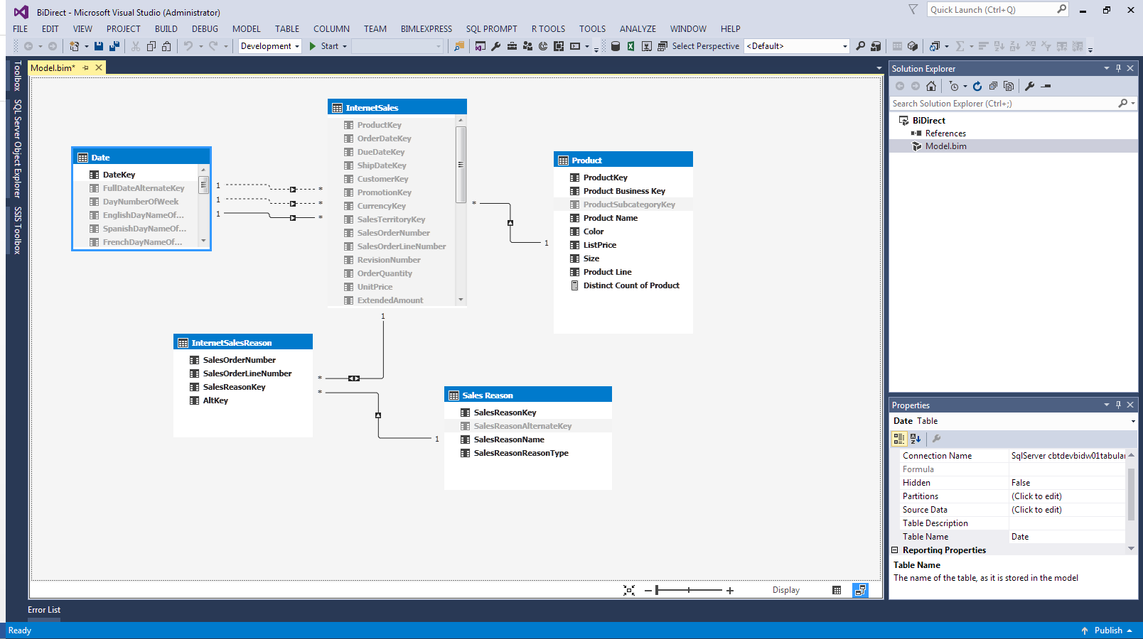
Figure 9 shows the Distinct Count of products with a filter on year for Internet Sales.
The Distinct Count is the same for all years, even years without any sales. Changing the relationship in the diagram view of the Tabular Model will solve this problem like Figure 10.
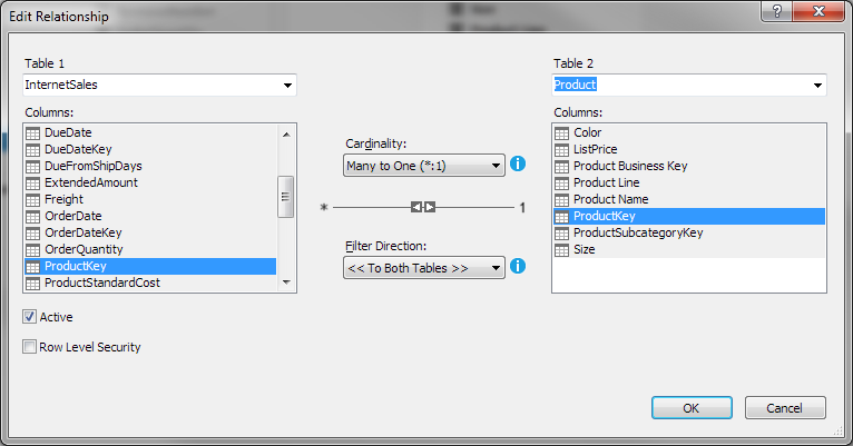
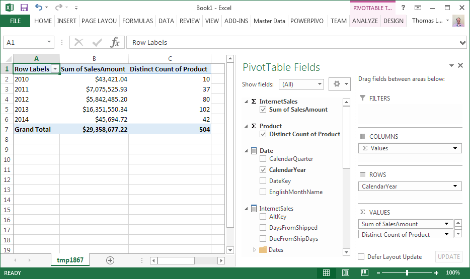
Figure 11 shows the Analyze in Excel results from using bi-directional filtering on the Production table relationship with the InternetSales table.
Analysis Services has been able to handle business logic like this in MDX and DAX. But users are more interested in these logical business rules to be implemented in the database. The Tabular Model is starting to look more and more like the Multidimensional Cube with the end result, not in the method of obtaining the result. Luckily there are plenty of users in the Microsoft Data Technology community willing to show how this works. Watch the new stuff coming in SQL Server 2017 and stay up with the changes.
Resources
- Define a Many-to-Many Relationship and Many-to-Many Relationship Properties
- Many-to-Many Relationships in the Data Warehouse
- Design Tip #142 Building Bridges

Starting as a developer in COBOL while at LSU, he has been a developer, tester, project manager, team lead as well as a software trainer writing documentation. Involvement in the SQL Server community includes speaking at SQLPASS.org Summits and SQLSaturday since 2011 and has been a speaker at IT/Dev Connections and Live! 360.
Currently, he is the Chair of the PASS Excel Business Intelligence Virtual Chapter and worked on the Nomination Committee for PASS Board of Directors for 2016.
View all posts by Thomas LeBlanc
- Performance tuning – Nested and Merge SQL Loop with Execution Plans - April 2, 2018
- Time Intelligence in Analysis Services (SSAS) Tabular Models - March 20, 2018
- How to create Intermediate Measures in Analysis Services (SSAS) - February 19, 2018