T-SQL as an asset to set-based programming approach

Introduction

This article is the third and last one of a series of articles that aims to introduce set-based programming approach inside SQL Server, so using Transact SQL. In first article “An introduction to set-based vs procedural programming approaches in T-SQL”, we’ve compared procedural and set-based approaches and came to the conclusion that the second one can facilitate developer or DBA’s life. In second article “From mathematics to SQL Server, a fast introduction to set theory”, we’ve made the parallel between mathematical definition of set theory and its implementation in SQL Server. Now, we’ll discuss about some other features from T-SQL that can’t be left aside when considering sets.

After some reminder from previous articles, we will look at different kinds of ways to combine records in tables using join operations. Then, we will cover a very useful feature called “common tabular expression”. Finally, we will implement or discuss solutions to real life problems.

Reminder from previous articles

A set is defined as a collection of elements.

A finite number of sets can be graphically represented using a Venn diagram.

Theoretical examples will use notation A and B for general sets or tables.

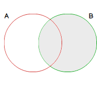
Following convention will be used for these examples: A is represented by red circle while green circle represents Set B. The results of an operator is the grayscaled parts of those circles.

More concrete examples that do not use A and B notation are also provided and built using Microsoft’s AdventureWorks database.

A SQL join is an operation that allows row combination from two or more tables.

SQL join operations

Overview

In the second article of this series “From mathematics to SQL Server, a fast introduction to set theory”, we’ve already seen a cross join operation which generates all possible combinations of the elements of two sets. Actually, this is not the only join operation we can use in SQL Server. In contrast to cross join, these other join operations need the definition of a condition for join operation execution to lead to the addition of a row in its results set. We will refer to this condition as the join condition. Most often, this join condition is built on key columns of tables implied in join operation.

Let’s now consider these other joins.

The typical join: INNER JOIN

The INNER JOIN is a join that only adds to its results set rows of both tables that lead to a true value for its join condition. This join condition is most often an equality condition on key columns.

In T-SQL, it looks like follows:

SELECT *

FROM A

INNER JOIN B

ON <join_condition>

Note

It’s sometimes referred to as self-join when a table is “self-joined” to itself.

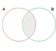
As only records matching join condition in both table are kept, an INNER JOIN can be represented by following figure. Let red circle be the set of records of A and the green one records of B both identified by the columns used in join condition, this operation can be seen as equivalent to the intersection between two sets.

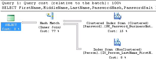
You will find below an example query that returns some person information with its password hash and salt.

SELECT

FirstName,

MiddleName,

LastName,

PasswordHash,

PasswordSalt

FROM Person.Person p

INNER JOIN Person.Password pp

ON pp.BusinessEntityID = p.BusinessEntityID

In this case, we only get results for persons defined in both Person and in Password tables. Here is the execution plan associated with the above query:

LEFT (OUTER) JOIN

A LEFT OUTER JOIN operation between table A and table B is a join that produces a set made up with rows of table A in conjunction with the matching rows of table B when join condition is met, i.e. when the value of join condition lead to a true value for those rows. For rows from table B that do not match join condition, SQL Server will set NULL values for columns from table B and append them to non-matching rows from the table A then add them to the results of this join operation.

We will use following notation to use this join.

SELECT *

FROM A

LEFT JOIN B

ON <join_condition>

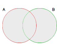
As all records from table A will be found as part of the results of a LEFT JOIN operation, it can be represented as follows:

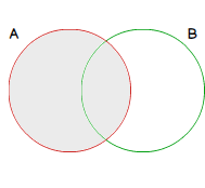
In AdventureWorks database, if we want to get all business entities and get persons information based on the value of BusinessEntityId column, we could get records with data from BusinessEntity table and NULL value for other columns.

SELECT *

FROM Person.BusinessEntity be

left join Person.Person p

on be.BusinessEntityID = p.BusinessEntityID

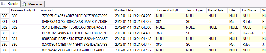
Sample results of this query:

RIGHT OUTER JOIN

The right outer join operation is the same as left outer join except that roles of tables are reversed: it takes from rows from the table B and appends columns from the table A when matching join condition and NULL otherwise.

We use this operator as follows:

SELECT *

FROM A

RIGHT JOIN B

ON <join_condition>

As all key columns from table B used in join condition will be in results set, it can be represented as this:

FULL OUTER JOIN

A FULL OUTER JOIN is the combination or the UNION (see second article of the series) of a LEFT OUTER JOIN and a RIGHT OUTER JOIN. For this reason, we will get both matching and non-matching rows from both tables.

We could represent the results set of FULL OUTER JOIN operation as follows:

Common tabular expressions (CTE)

Overview

Common tabular expression or CTE is a feature introduced in SQL Server since its 2005 version. You can think of it as a temporary results set loaded at execution in a single data management T-SQL statement.

As it’s defined inside a DML statement:

CTE is not an object and does not need to be created or dropped.
Its data are not kept after statement execution
Can be referenced, even in itself (self-referencing)

CTE can be used in multiple use cases:

Replacement for a view
Building a recursive query
Reference results set of a query multiple times in the same statement
…

Common tabular expression is an unavoidable element in set-based programming as it defines a set we can use in a statement.

We will now have a look at its structure and we will notice directly that it becomes very handy in terms of readability and, de facto, of complex query maintenance.

Structure of a query using CTE

A DML query that uses a common tabular expression always starts with the « WITH » keyword followed by a nickname or an alias for CTE’s subquery. Optionally, we can define column names for CTE columns when they will not be defined in a subquery. Then comes CTE’s subquery itself enclosed by parentheses. Note that we can chain CTE by replacing WITH keyword by a comma in subsequent CTE definitions. Finally comes the DML query itself.

In pseudo-code:

WITH expression_name [ ( column_name [,...n] ) ]

AS (

CTE_query_definition

)

[, Additional_CTE_definitions ]

DML_query

Example usage 1: Non-recursive query

Let’s review our first example. In this example, we will list records from Person table that did not change their password since at least a year.

To do it, we will first get the list of passwords with LastModifiedDate column with a value older than 365 days. This can be performed by following query:

SELECT BusinessEntityID, ModifiedDate as LastPwdChangeDate

FROM Person.Password

WHERE DATEDIFF(DAY,ModifiedDate,GETDATE()) > 365

;

Now we have built a query that provides us the set of values of identifiers of interest. We can define this query as a CTE we will call UsersWithOldPassword .

We can now take the list of persons based on the value of BusinessEntityId column from our CTE. To do so, we will use the INNER JOIN operation presented above.

Final query will look like follows:

WITH UsersWithOldPassword

AS (

SELECT

BusinessEntityID,

ModifiedDate as LastPwdChangeDate

FROM Person.Password

WHERE DATEDIFF(DAY,ModifiedDate,GETDATE()) > 365

)

SELECT

p.BusinessEntityID,

p.FirstName,

p.MiddleName,

p.LastName,

uwop.LastPwdChangeDate

FROM Person.Person p

INNER JOIN

UsersWithOldPassword uwop

ON p.BusinessEntityID = uwop.BusinessEntityID

This simple example shows the advantages of using CTE: we can create subqueries, test them, then use them to provide final results.

Example 2: recursive query

Recursive CTE are very handy to manage the hierarchical relationship between data. You will find below a list of different examples that come to my mind when I talk about recursive CTE:

Generate a tree representation of process blocking chain (for DBAs)
Generate the complete path of a directory from a hierarchically defined DirectoryPath table
Generate a set of ordered numbers
Generate effective permissions for a given SQL login or database user (for DBAs)
Checking an application user can actually access a resource (when the application uses an authorization system involving roles)
…

As you can see, they are many applications to recursive CTE. We won’t review each of them, but we will focus on an example based on AdventureWorks database (for consistency). Details about this example will be explained at the appropriate moment.

But before talking about it, you will find hereby the general syntax used to build a recursive common tabular expression:

WITH NameOfTheCTE (ColumnA, ColumnB, …)

AS (

QueryDefinition_NoRecursion

UNION ALL

QueryDefinition_WithRecursion -- references NameOfTheCTE.

)

-- Statement using the CTE

SELECT *

FROM NameOfTheCTE

This way of building a recursive CTE reminds me my days at school where we had to demonstrate the formula of a series or recursive sums. We were used to start with a definition of one or more initial values of the series before considering the formula as thesis.

Here, it’s kind of the same thing: we will consider sets that do not need recursion to produce results (the Initial Set) then take the union of this initial set with the results from a query that uses the CTE we are defining (the Recursive Call). By the way, we need to tell SQL Server where to stop in its recursion. It’s the recursion stop condition. Finally, we reference the CTE inside the DML query.

Before diving into the actual example this section, we will take a closer look at an example recursive CTE that generates 30 numbers.

WITH NumEnum

AS (

SELECT 1 as N -- <----------- INITIAL SET

UNION ALL

SELECT N+1 as N -- <----------- RECURSIVE CALL

FROM NumEnum

WHERE N < 30 -- <----------- RECURSION STOP CONDITION

)

SELECT N -- <----------- CTE INVOCATION

FROM NumEnum

Note

SQL Server limits the depth of recursion. By default, this depth is limited to 100. When this limit is reached, we will get following message:

Now, it’s time to explain the example we will use in this section. We will consider Production.Product and Production.BillOfMaterials tables.

First, let’s review some information about Product table. This information is taken from technet.

This table lists information about each product sold by Adventure Works Cycles or used to manufacture Adventure Works Cycles bicycles and bicycle components.

And now, let’s consider information about BillOfMaterials table:

This table lists of all the components used to manufacture bicycles and bicycle subassemblies.
The ProductAssemblyID column represents the parent, or primary, product and ComponentID represents the child, or individual, parts used to build the parent assembly.
The BOM_Level column indicates the level of the ComponentID relative to the ProductAssemblyID.
An EndDate column with a value means that component stopped being used to assemble product.

So, basically, we can identify a Parent-Child relationship and an application like getting the list of a product sub-assemblies and parts that compose these assemblies.

To do so, we will write a CTE called MaterialDetails. This CTE will be defined with the following columns:

ProductId
ProductNumber,
ProductName,
MaterialQuantity,
ProductColor,
HierarchyDepth,
ProductAssemblyId
ProductNamePath

So, first part of CTE will be as follows:

WITH MaterialDetails (

ProductId, ProductNumber, ProductName, MaterialQuantity,

ProductColor, HierarchyDepth, ProductAssemblyId, ProductNamePath

)

AS (

Now, let’s build the initial set list. It’s done by getting the list of products that have a row in BillOfMaterials table with no parent assembly, so with ProductAssemblyId column set to NULL. We also need to filter out those materials that are not used anymore in the assembly of the product.

Here is the query to do so.

SELECT

p.ProductID,

p.ProductNumber,

p.Name,

CAST (1 AS DECIMAL (10, 2)),

p.Color,

NULL,

CAST(P.Name AS VARCHAR(128))

FROM

Production.Product AS p

INNER JOIN

Production.BillOfMaterials AS bom

bom.ComponentID = P.ProductID

AND bom.ProductAssemblyID IS NULL

AND (

bom.EndDate IS NULL

OR bom.EndDate > GETDATE()

)

;

Now, we have the initial set. As we will want to cross hierarchy of product assembly, it should be handy to generate a tree view of this hierarchy. To do so, we will append a string per hierarchy level to the name of sub-assembly.

So, the recursive call should look like follows:

SELECT

-- current product informations

p.ProductID,

p.ProductNumber,

-- hierarchical tree visualization

CAST (REPLICATE(' ', md.HierarchyDepth - 1)

+ '|--- ' + P.Name AS VARCHAR (8000)),

-- current assembly quantity

bom.PerAssemblyQty,

-- current product color (when applicable)

p.Color,

-- we go deeper in hierarchy so...

md.HierarchyDepth + 1,

-- keep reference of current product identifier

md.ProductId,

-- this is for display

CAST(md.ProductNamePath + '\' + p.Name AS varchar(MAX))

FROM

-- take back last recursion results

MaterialDetails AS md

-- retrieve informations about current level of details

INNER JOIN

Production.BillOfMaterials AS bom

ON md.ProductId = bom.ProductAssemblyID

INNER JOIN

Production.Product AS p

on p.ProductID = bom.ComponentID

-- don't forget some parts may not be used anymore

WHERE (

bom.EndDate IS NULL

OR bom.EndDate > GETDATE()

)

The invocation of CTE is pretty easy as it will just be a SELECT statement from that CTE.

SELECT

ProductId,

ProductNumber,

ProductName,

MaterialQuantity,

ProductColor,

HierarchyDepth,

ProductAssemblyId,

ProductNamePath

FROM MaterialDetails

Putting all these parts together, CTE will look like this:

WITH MaterialDetails (

ProductId, ProductNumber, ProductName, MaterialQuantity,

ProductColor, HierarchyDepth, ProductAssemblyId, ProductNamePath

)

AS (

SELECT

p.ProductID,

p.ProductNumber,

CAST(p.Name AS varchar(8000)),

CAST (1 AS DECIMAL (8, 2)),

p.Color,

NULL,

CAST(P.Name AS VARCHAR(MAX))

FROM

Production.Product AS p

INNER JOIN

Production.BillOfMaterials AS bom

bom.ComponentID = P.ProductID

AND bom.ProductAssemblyID IS NULL

AND (

bom.EndDate IS NULL

OR bom.EndDate > GETDATE()

)

UNION ALL

SELECT

-- current product informations

p.ProductID,

p.ProductNumber,

-- hierarchical tree visualization

CAST (REPLICATE(' ', md.HierarchyDepth - 1) + '|--- ' + P.Name AS VARCHAR (8000)),

-- current assembly quantity

bom.PerAssemblyQty,

-- current product color (when applicable)

p.Color,

-- we go deeper in hierarchy so...

md.HierarchyDepth + 1,

-- keep reference of current product identifier

md.ProductId,

-- this is for display

CAST(md.ProductNamePath + '\' + p.Name AS varchar(MAX))

FROM

-- take back last recursion results

MaterialDetails AS md

-- retrieve informations about current level of details

INNER JOIN

Production.BillOfMaterials AS bom

ON md.ProductId = bom.ProductAssemblyID

INNER JOIN

Production.Product AS p

on p.ProductID = bom.ComponentID

-- don't forget some parts may not be used anymore

WHERE (

bom.EndDate IS NULL

OR bom.EndDate > GETDATE()

)

SELECT

ProductId,

ProductNumber,

ProductName,

MaterialQuantity,

ProductColor,

HierarchyDepth,

ProductAssemblyId,

ProductNamePath

FROM MaterialDetails

ORDER BY ProductNamePath

;

Here is a sample of the results of the query:

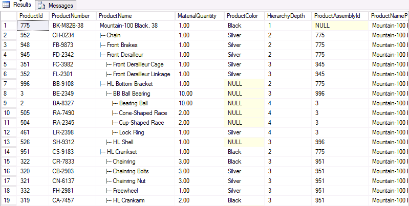
If we would like to implement this function inside an application using procedural approach, we would have needed to write a lot more code involving at least the use of a cursor for initial step, a loop to read products from that cursor, a temporary table to insert results on the fly and a lot more. We could expect this solution to take so much more time and consume so much more resources compared to set-based solution.

Advanced examples

Generate all seconds in a day

I already talked about an example usage for set-based approach which can be used to generate charts for data from your homemade monitoring tool. I use to save disk space and whenever possible, I log only occurrences of an event, not the absence of event with a timestamp corresponding to the moment it occurred.

So, I’m used to have tables with following structure:

DateStamp DATETIME, <SpecificMonitoredData>

It’s a good candidate to generate charts with time as X axis and either a specific value (like the total RAM used) or the number of occurrences of the event as Y axis.

But, as I already explained previously, there can be holes in the data. If we want to plug that hole for a given day, we will use recursive CTE to generate all the X axis values and join them with data from monitoring using an INNER JOIN.

So, we will have a fixed date in short format (yyyymmdd) and cross join it with a set of 24 numbers from 0 to 23 (for hours) and cross join it with a set of 60 numbers from 0 to 59 (for minutes) and cross join it once more with 60 numbers from 0 to 59 (for seconds).

Instead of using former query to generate these numbers, we will use following CTE:

WITH NumberCollection (

)

AS (

SELECT ROW_NUMBER()

OVER (ORDER BY (SELECT NULL))

FROM sys.all_columns a

CROSS JOIN sys.all_columns b

)

Following query will give you exactly what we need to perform the INNER JOIN with the monitoring history table.

WITH DayOfInterest

AS (

SELECT

convert(varchar(8), getdate(), 112) as DateShort

NumberCollection (

)

AS (

SELECT ROW_NUMBER()

OVER (ORDER BY (SELECT NULL))

FROM sys.all_columns a

CROSS JOIN sys.all_columns b

Hourly

AS (

SELECT TOP 24 N from NumberCollection

MinuteAndSecondsly

AS (

SELECT TOP 60 N FROM NumberCollection

)

select

DayOfInterest.DateShort,

RIGHT('0000' + CONVERT(varchar(4),Hourly.N),2) AS HourCount,

RIGHT('0000' + CONVERT(varchar(4),Minutely.N),2) AS MinutesCount,

RIGHT('0000' + CONVERT(varchar(4),Secondly.N),2) AS SecondsCount

FROM DayOfInterest,

Hourly,

MinuteAndSecondsly as Minutely,

MinuteAndSecondsly as Secondly

As this generation of all seconds in a day can be time consuming, we could create a TimeDimension table and use it directly in hour developments.

Generate a calendar table

Calendar table have been explained by Ed Pollack in his articles series which first article is entitled Designing a Calendar Table. In short, it’s a table with dates and some data around dates. While he explains very well this concept, the stored procedure he defined to populate this table is designed using procedural approach. This stored procedure takes two parameters: StartDate and EndDate.

An alternative to his procedure would use a CTE composed with the definition of NumberCollection and another query that would generate dates between the values of these parameters.

Here is the beginning of a solution:

DECLARE @StartDate DATETIME = GETDATE() - 10 ;

DECLARE @EndDate DATETIME = GETDATE() + 10 ;

WITH NumberCollection (

)

AS (

SELECT ROW_NUMBER()

OVER (ORDER BY (SELECT NULL))

FROM sys.all_columns a

CROSS JOIN sys.all_columns b

NbDaysOfInterest

AS (

SELECT TOP (DATEDIFF(DAY,@StartDate,@EndDate))

FROM NumberCollection

DatesOfInterest (

DateShort

)

AS (

SELECT CONVERT(VARCHAR(12),@StartDate + N,112)

FROM NbDaysOfInterest

WHERE @StartDate + N <= @EndDate

)

SELECT *

FROM DatesOfInterest

;

Summary

In this series of articles, we’ve seen that we can get benefit to implement solutions to complex problems using set-based programming approach. You will find below a final table with all the different T-SQL commands we’ve reviewed.

Procedural Approach	Set-Based Approach
SELECT and other DML operations, WHILE, BREAK, CONTINUE, IF…ELSE, TRY…CATCH Cursors (OPEN, FETCH, CLOSE) DECLARE	SELECT and other DML operations, Aggregate functions (MIN, MAX, AVG, SUM…) UNION and UNION ALL EXCEPT and INTERSECT CROSS JOIN INNER JOIN [LEFT \| RIGHT \| FULL] OUTER JOIN, Common Tabular Expressions

As a final warning, I would like to insist on the fact that set-based programming approach is a very cool way to solve problems but it won’t be the answer to any problems. Instead, we can build “hybrid” solutions that are procedural by design, but really take advantage of set-based approach so that we get the best out of both.

SQLShack

T-SQL as an asset to set-based programming approach

Introduction

Reminder from previous articles

SQL join operations

Common tabular expressions (CTE)

Advanced examples

Summary

Further readings

Introduction

Reminder from previous articles

SQL join operations

Common tabular expressions (CTE)

Advanced examples

Summary

Further readings

Related posts: