
Introduction
In our SQLShack discussions over the past few weeks, we have dealt with a few of the more conventional SQL Server data manipulation techniques. Today we are going to be a bit more avant-garde and touch upon a subject dear to my heart.
With Power Bi becoming more and more important on the business side within major industries worldwide, it is not surprising that sooner or later every SQL programmer is going to have to learn and be able to ‘talk’ DAX.
In this article we are going to have a look at the a few of the more important ‘constructs’ and produce production grade queries for data extraction and for reports; enabling the reader to ‘hit the ground running’.
The Microsoft Business Intelligence Semantic Model (BISM)
Prior to any discussion pertaining to Data Analysis Expressions or DAX, it is imperative to understand that DAX is closely link to the Business Intelligence Semantic Model (hence forward referred to as the BISM). Microsoft describes the BISM as “a single model that serves all of the end-user experiences for Microsoft BI, including reporting analysis and dash boarding”.
In fact, in order to extract data from any tabular Analysis Services projects, the DAX language is the recommended language of choice. DAX itself is a rich library of expressions, functions that are used extensively within Microsoft Power Pivot and SQL Server Analysis Services tabular models. It is a ‘build out’ of Multi-Dimensional Expressions (MDX) and it does provide exciting new possibilities.
This said let us get started.
Installation of a Tabular Instance of SQL Server Analysis Services
With the advent of SQL Server 2012 and up, there are two flavors of Analysis Services:
- The Multidimensional Model
- The Tabular Model
Both of these models require separate instances. More often than not, for any project, I normally create a relational instance for run of the mill data processing and either a Tabular Instance or a Multidimensional Instance (depending upon the client/ project requirements). In short, one Analysis Services Instance cannot be both at the same time.
There is a way to change an instance to the opposite model (YES YOU CAN!!!) however it is NOT DOCUMENTED nor recommended by Microsoft. The main issue is that the server MUST BE stopped and restarted to move from one mode to the other.
To create a Tabular Instance simply create one with the SQL Server Media (BI edition or Enterprise edition 2012 or 2014). Install only the Analysis Services portion.
Getting started
SQL Shack industries has a relational database called DAXandTabularModel. A few months back they created a SQL Server Data Tools project to define and create their Tabular SalesCommissionReport Analysis Services database. The ins and outs of how this project was created is beyond the scope of this article however the project data may be seen below: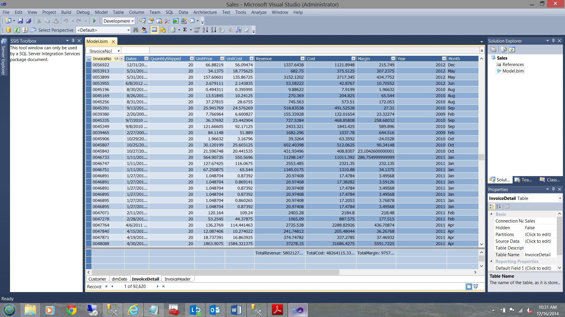
The project consist of four relational tables:
- Customer (containing customer details)
- dimDate (a Date entity with week number, month number, etc.)
- Invoice Header (the mommy a header has many details)
- Invoice Detail (the children)
This project model once deployed created the Analysis Services database with which we are now going to work.
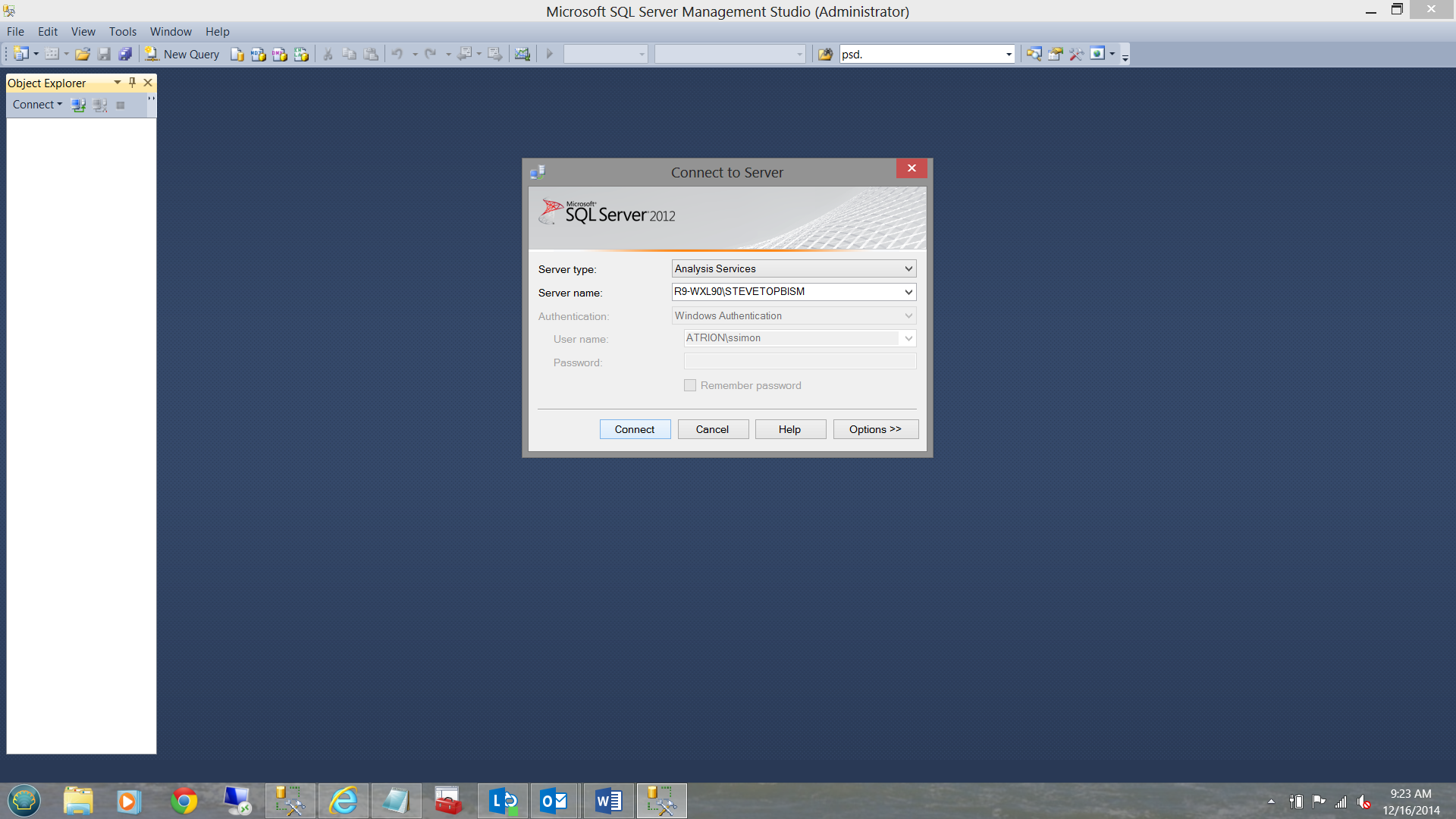
Let us begin by bringing up SQL Server Management Studio and log into a Tabular Instance that I have created.
As a starting point we are going to have a quick look at how simple DAX queries are structured.
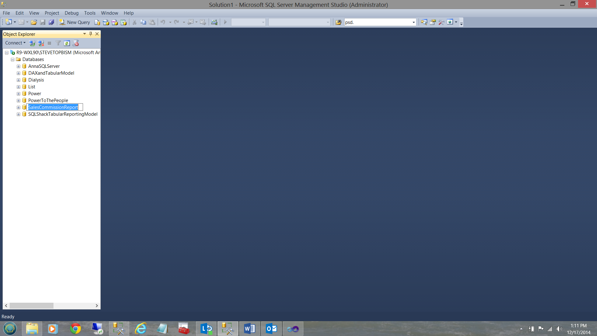
Having opened Analysis Services we note that there is a Tabular Analysis Services database called “SalesCommissionReport”. We shall be working with this database.
We now open a ‘New Query’ (see above).
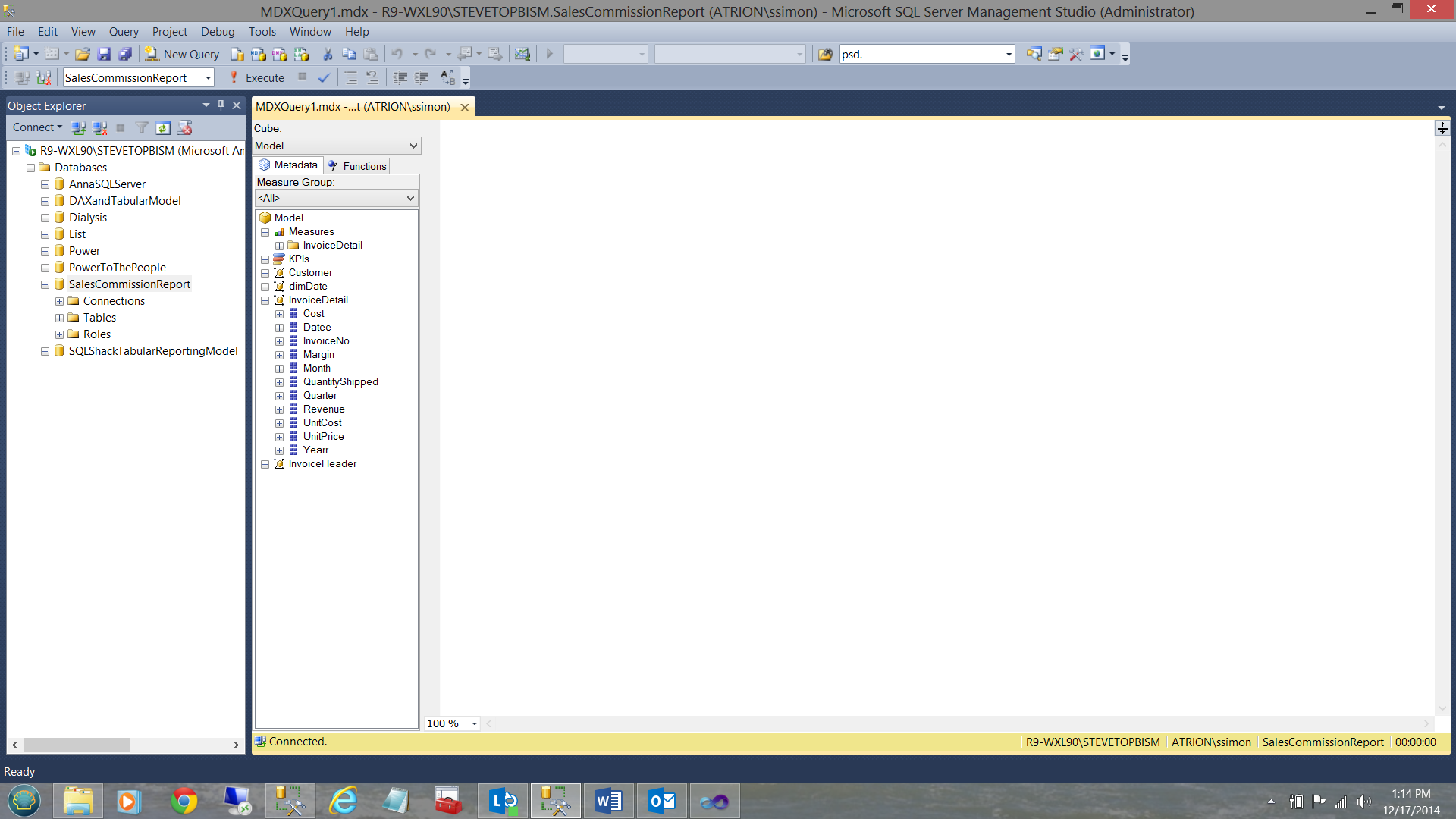
Note that the appearance of the query window is somewhat reminiscent of query work surface for multidimensional queries.
For our first example let us take a look at a simple business query.
SQLShack Industries wishes to ascertain the total revenue, total cost and total margin for the varied invoiced items for a given time period.
In T-SQL we could express this in the following manner:
|
1 2 3 4 5 |
Select InvoiceNo, Datee as [Date], sum(Revenue) as Revenue, sum(Cost) as Cost, Sum(Margin) as Margin from DaxAndTheTabularModel Group by InvoiceNo, Datee |
Now!! Let us now see (in easy steps) how we may construct this same query within the world of DAX.
To begin, we wish to create a piece of code that will sum the revenue, cost and margin. Let us see how this is done!
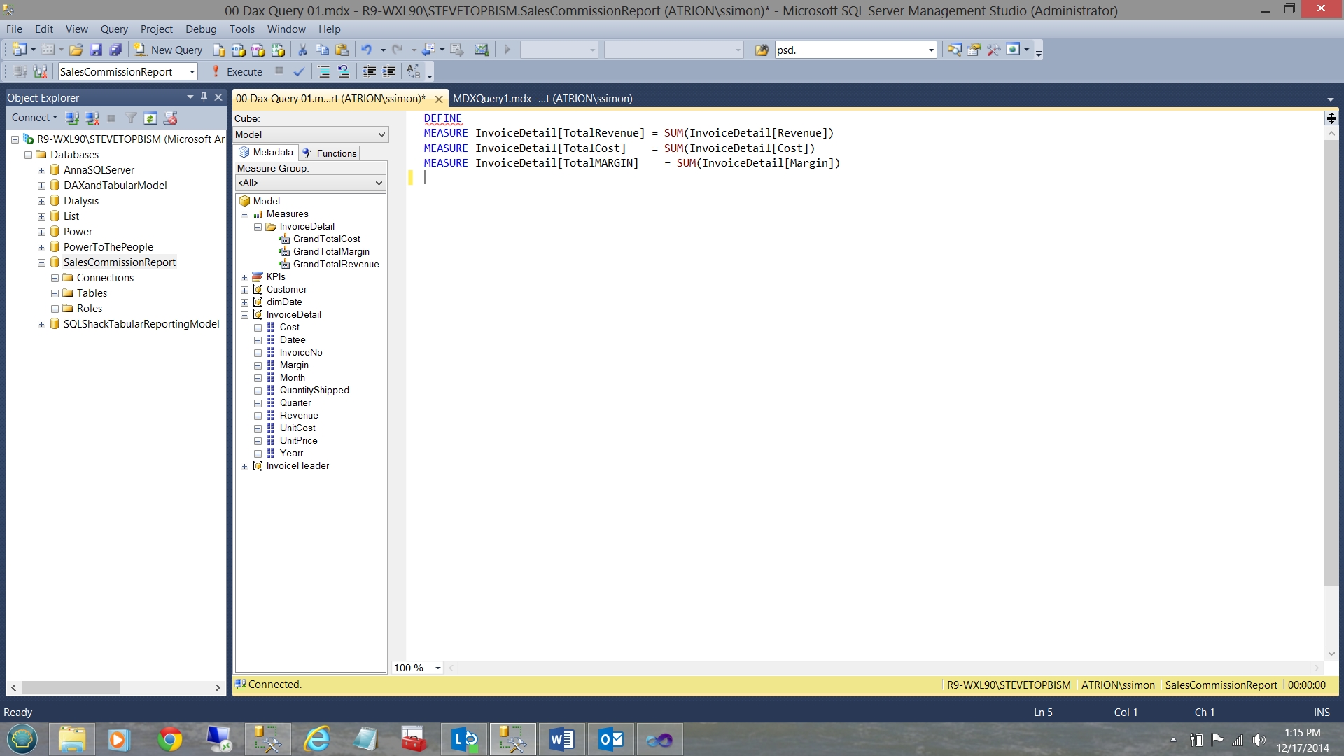
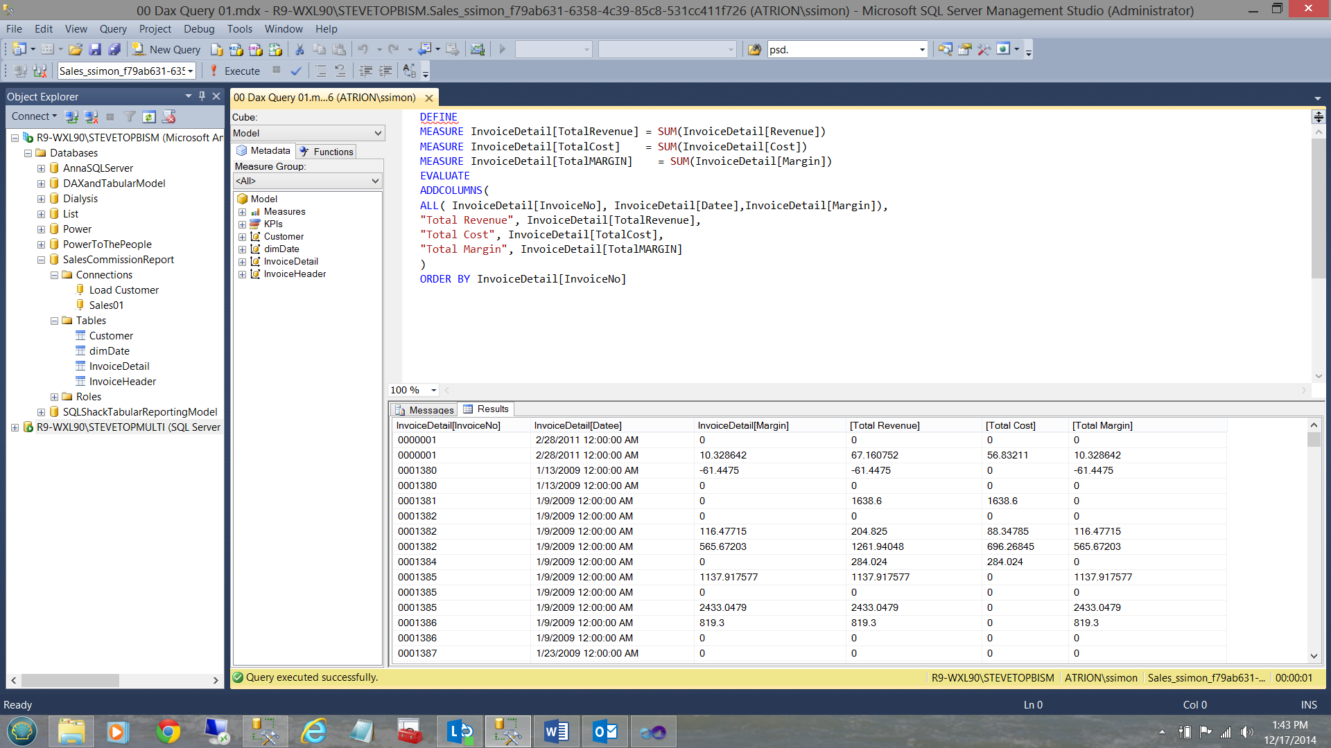
We note the command DEFINE at the start of the query. The astute reader will note that the ‘InvoiceDetail’ entity (see above) contains the fields “Revenue”, ”Cost” and “Margin”. These are the fields that we shall be using. Note that the three measures are created below the word DEFINE (see above (in the screen dump) and below for a snippet of the code).
|
1 2 3 4 5 6 |
DEFINE MEASURE InvoiceDetail[TotalRevenue] = SUM(InvoiceDetail[Revenue]) MEASURE InvoiceDetail[TotalCost] = SUM(InvoiceDetail[Cost]) MEASURE InvoiceDetail[TotalMARGIN] = SUM(InvoiceDetail[Margin]) |
A note is required at this point: The syntax for pulling fields from tabular databases is:
Entity[Attribute] as may be seen above. In our case “InvoiceDetail” is the entity and [TotalRevenue] the attribute.
Now that we have created our ‘DEFINED’ fields it is time to construct the main query.
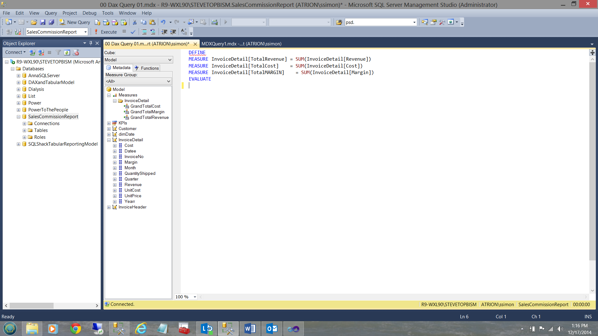
We first add the word ‘EVALUATE’ below our declaration of the MEASURES. EVALUATE corresponds to the word SELECT in traditional SQL code.
Having issued the “EVALUATE” we now call for the fields that we wish to show within our query
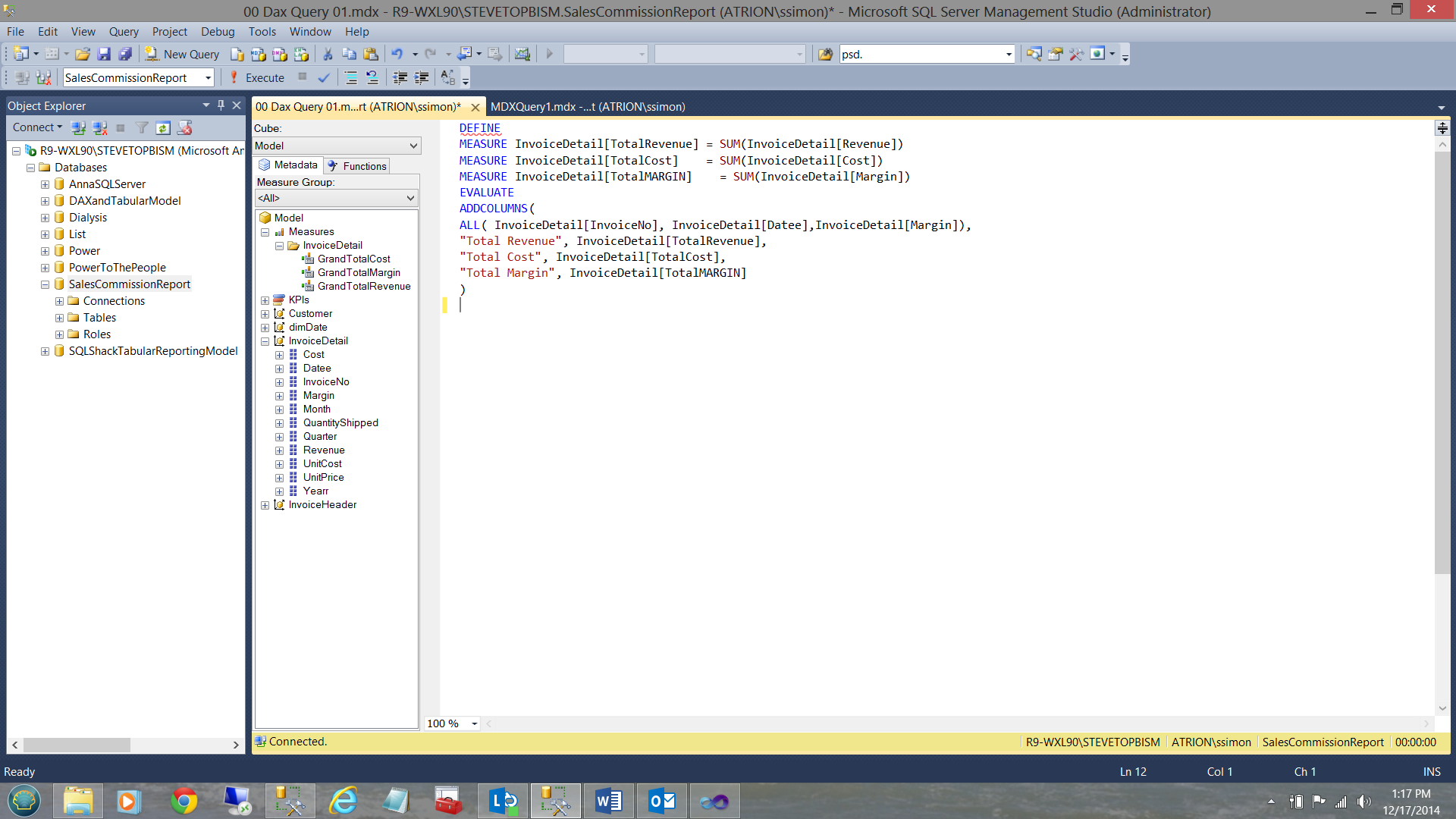
Note that we utilize the ADDCOLUMNS function to achieve this. The columns within the query may be seen above and a snippet of code may be seen below:
|
1 2 3 4 5 6 7 8 |
ADDCOLUMNS( ALL( InvoiceDetail[InvoiceNo], InvoiceDetail[Datee],InvoiceDetail[Margin]), "Total Revenue", InvoiceDetail[TotalRevenue], "Total Cost", InvoiceDetail[TotalCost], "Total Margin", InvoiceDetail[TotalMARGIN] ) |
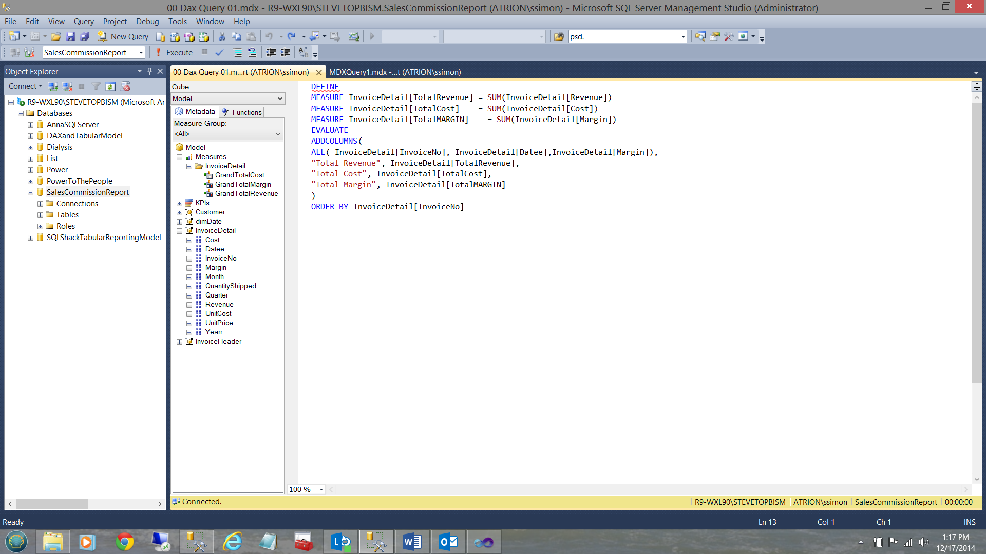
To complete the code and knowing that I want the data ordered by the invoice number, I add an ORDER BY statement.
|
1 2 3 |
ORDER BY InvoiceDetail[InvoiceNo] |
Thus our query is complete. Let us give it a spin!!
The results of the query may be seen below.
To recap
- DEFINE
- Create your define fields
- ADDCOLUMNS to your query including the defined fields
- Order by statement.
We shall see how to use this for constructive usage in a few minutes.
Another Example:
In the next example I want to show you how easily one may obtain data from two or more entities (tables).
After all in the real world, reporting queries normally do join to two or more tables. In our case we wish to look at ONLY data from the year 2010.
Once again we start with the necessary EVALUATE command. We remember from above that this is the equivalent to the SELECT statement.
This time however we are going to utilize the “CALCULATETABLE” function. “CALCULATETABLE” evaluates a table expression in a context modified by the given filters (see below in yellow)
|
EVALUATE
CALCULATETABLE(
SUMMARIZE(
‘InvoiceDetail’,
‘dimDate’[datee],
‘Customer’[CustomerName],
"Sales", SUM( Invoicedetail[Revenue] )
),
InvoiceDetail[Yearr] = 2010
)
order by ‘Customer’[CustomerName],‘dimDate’[datee]
|
The astute reader will note that I am pulling the date from the ‘InvoiceDetail’ table (after all, an item is sold on a given date, not so? The customer name from the “Customer” table and the field “Sales” is sourced from the “InvoiceDetail” table.
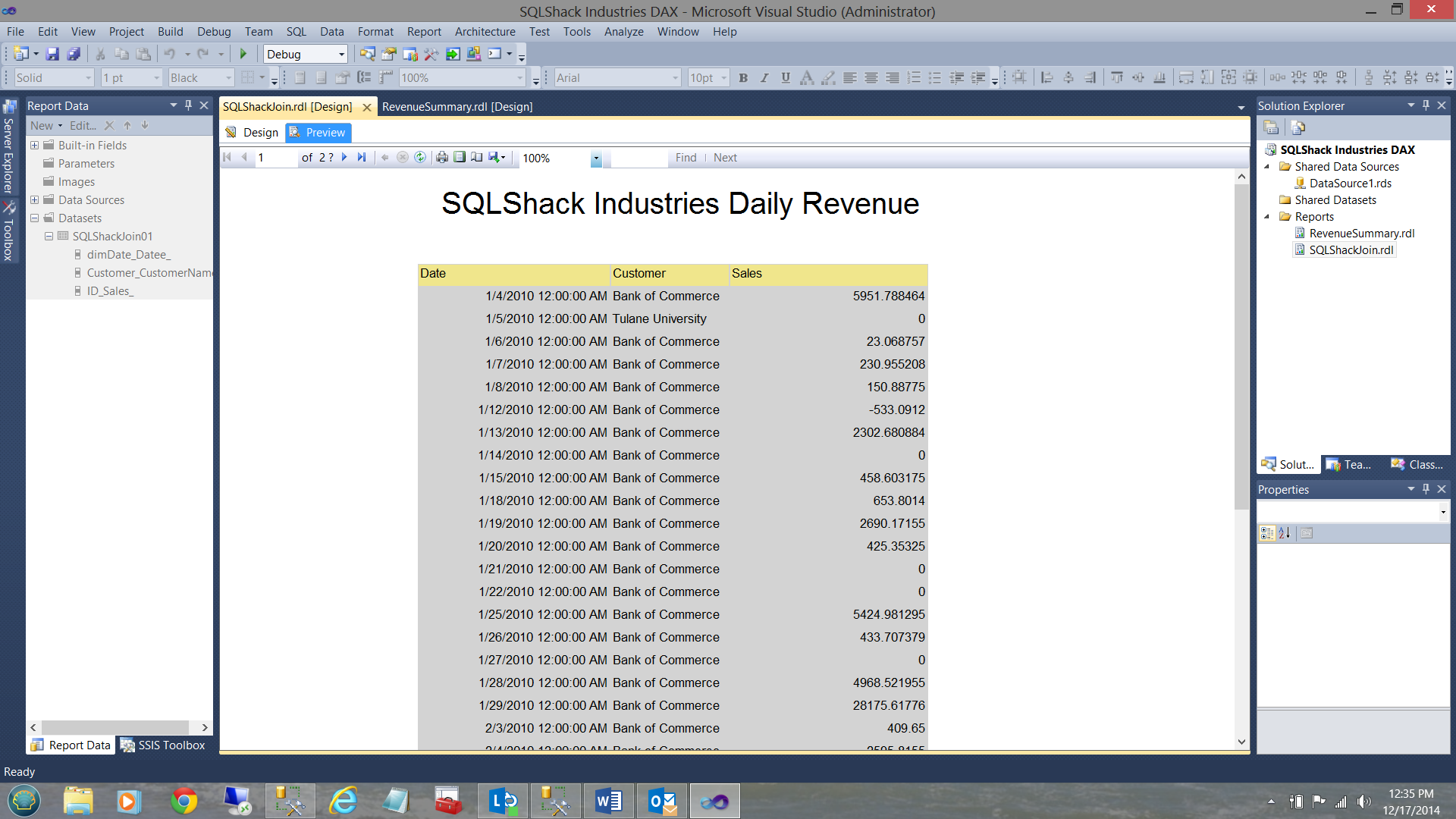
When we run our query we find the following:
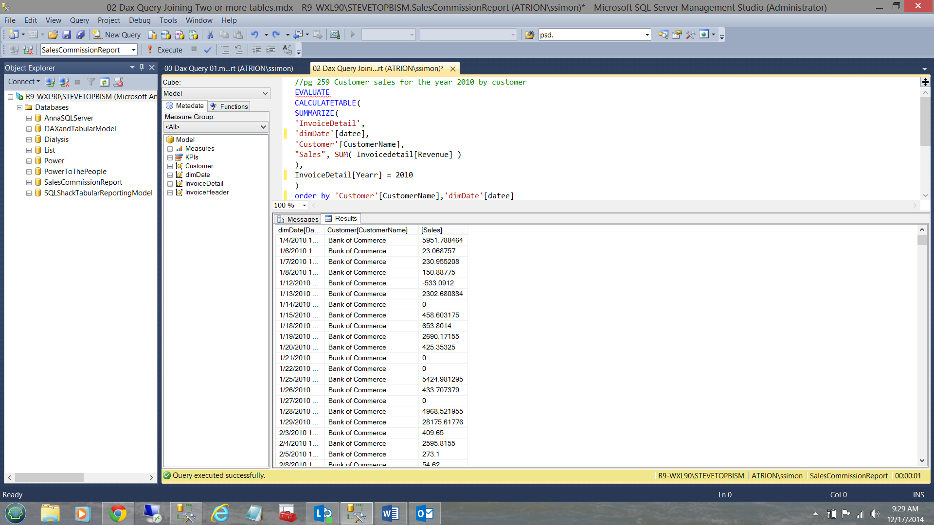
Normally SQLShack Industries work solely with an invoice date only as opposed to the date and time. Often the time is meaningless as it is 00:00:00 etc. Invoice date and dollar values with thousandths and millionth of cents is also nonsense UNLESS one is in the banking industry. This said we shall “normalize” these values when we come to the report section of this article.
One of my FAVORITE queries
One of the most beautiful features of using DAX is the ability to ascertain values for “the same period last year”.
In this query we are going to once again SUMMARIZE ( sum() ) the values and add the columns. This one however is a tad tricky to understand thus I am going to put the query together in pieces.
Firstly, here are my DEFINE fields
|
1 2 3 4 5 6 |
DEFINE MEASURE 'Invoicedetail'[CalendarYear] =sumx('dimDate',Year('dimDate'[datee]) ) MEASURE 'InvoiceDetail'[PY Sales] = CALCULATE( sumx('InvoiceDetail','Invoicedetail'[Revenue]), SAMEPERIODLASTYEAR( 'dimDate'[Datee] )) |
The first line of code will give us the calendar year in which the items were sold. This helps the folks at SQLShack Industries set their frame of reference.
The next line of code is a bit convoluted however simply put “PY Sales” is defined as ‘InvoiceDetail’[Revenue] FOR THE SAME DATE AND MONTH LAST YEAR! This is where the function
|
1 |
SAMEPERIODLASTYEAR( 'dimDate'[Datee] ) |
comes into play.
Let us finally proceed to add our query columns so that we can view the result set of the query.
|
1 2 3 4 5 6 7 8 9 10 11 12 13 14 15 16 17 18 19 20 |
EVALUATE ADDCOLUMNS( FILTER<strong>(</strong> SUMMARIZE<strong>(</strong> 'dimDate', 'dimDate'[datee], 'dimDate'[Month], 'dimDate'[Quarter], 'dimDate'[Weeknumber] ,"Sales: Today", sumx('InvoiceDetail','Invoicedetail'[Revenue]), "Calender Year" ,'Invoicedetail'[CalendarYear] ), //Filter the data sumx('InvoiceDetail','Invoicedetail'[Revenue]) <> 0 ), // Add the past period DEFINED column "Sales: Year ago Today", [PY Sales] ) ORDER BY 'dimDate'[Datee], 'dimDate'[Month] |
Once again, let us look at what each line of code achieves.
Under “SUMMARIZE”, from the dimDate entity (table), pull the date, month, quarter and week number of the invoice date.
THEN
|
1 |
"Sales: Today", sumx('InvoiceDetail','Invoicedetail'[Revenue]), |
Sum the revenue for the date ( i.e. sum(revenue) group by date) for the CURRENT year under consideration.
We must remember that where current invoice year is 2012 then we create our “Last Year’s field” from the same date but for the year 2011. The important point being that aside from the lowest year’s data, EACH invoice date ‘has a turn’ to be a current date and the ‘same day and month’ BUT one year earlier (see the table below).
| Prior Year | Current Year |
| 20100101 | 20110101 |
| 20090101 | 20100101 |
| NULL | 20090101 |
We also add the calendar year under consideration so that we know where we are in our table.
As a means of showing how to create a query predicate, I am including a filter within this code. It probably does NOT make any business sense and is meant purely to be demonstrative.
|
1 2 3 |
//Filter the data sumx('InvoiceDetail','Invoicedetail'[Revenue]) <> 0 |
Finally, I add the revenue from the prior period. NOTE that this is OUTSIDE of the SUMMARIZE function and the reason for this, is to avoid applying the conditions set within the SUMMARIZE function to the prior year’s figures.
|
1 2 |
"Sales: Year ago Today", [PY Sales] |
Finally we order our result set(by year, by month)
|
1 |
ORDER BY 'dimDate'[Datee], 'dimDate'[Month] |
Having now created three queries and knowing that we could have created a plethora more, at this point in time we should now have a look at how these queries may be utilized in a practical reporting scenario.
Creating reports with DAX queries
We start (as we have in past discussions) by opening SQL Server Data Tools and by creating a new Reporting Services project. Should you be a bit uncertain how to create a Reporting Services project, please have a glance at one of my earlier articles where I do describe the project creation in detail OR contact me directly for some super “crib” notes!
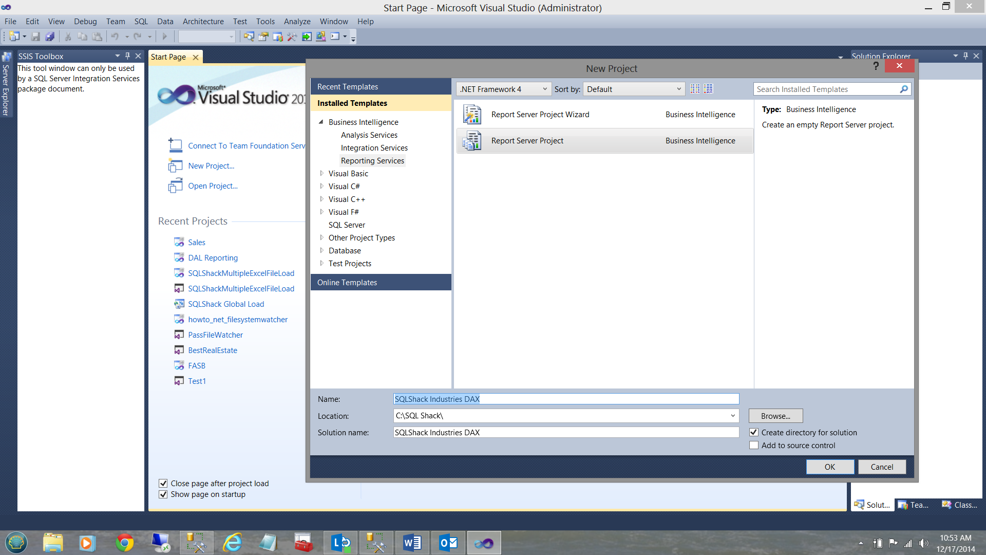
We click OK to create the project. Once within the project, we right click on the “Report” folder and select “Add” and then “New Item” (see below).
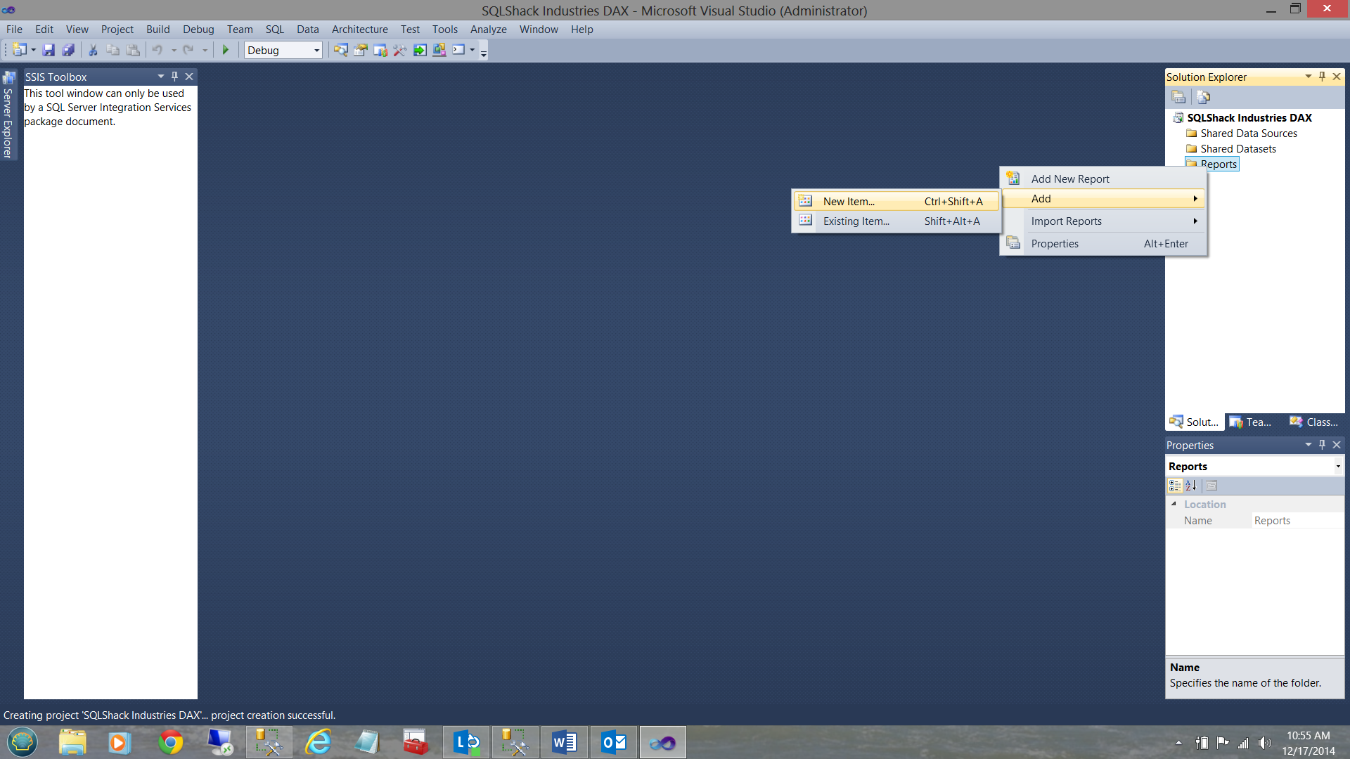
The new item report screen is then brought into view (see below).
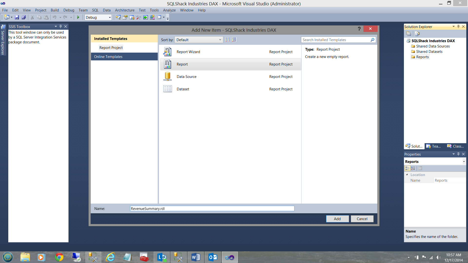
I select “Report” , give my report a name and the click “Add”.
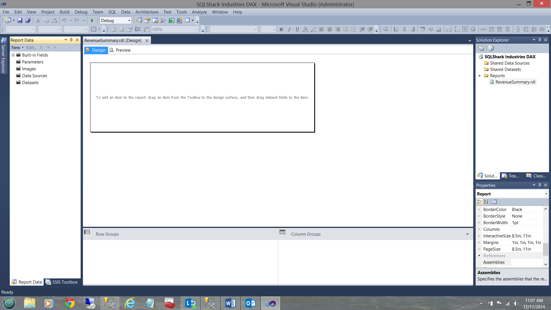
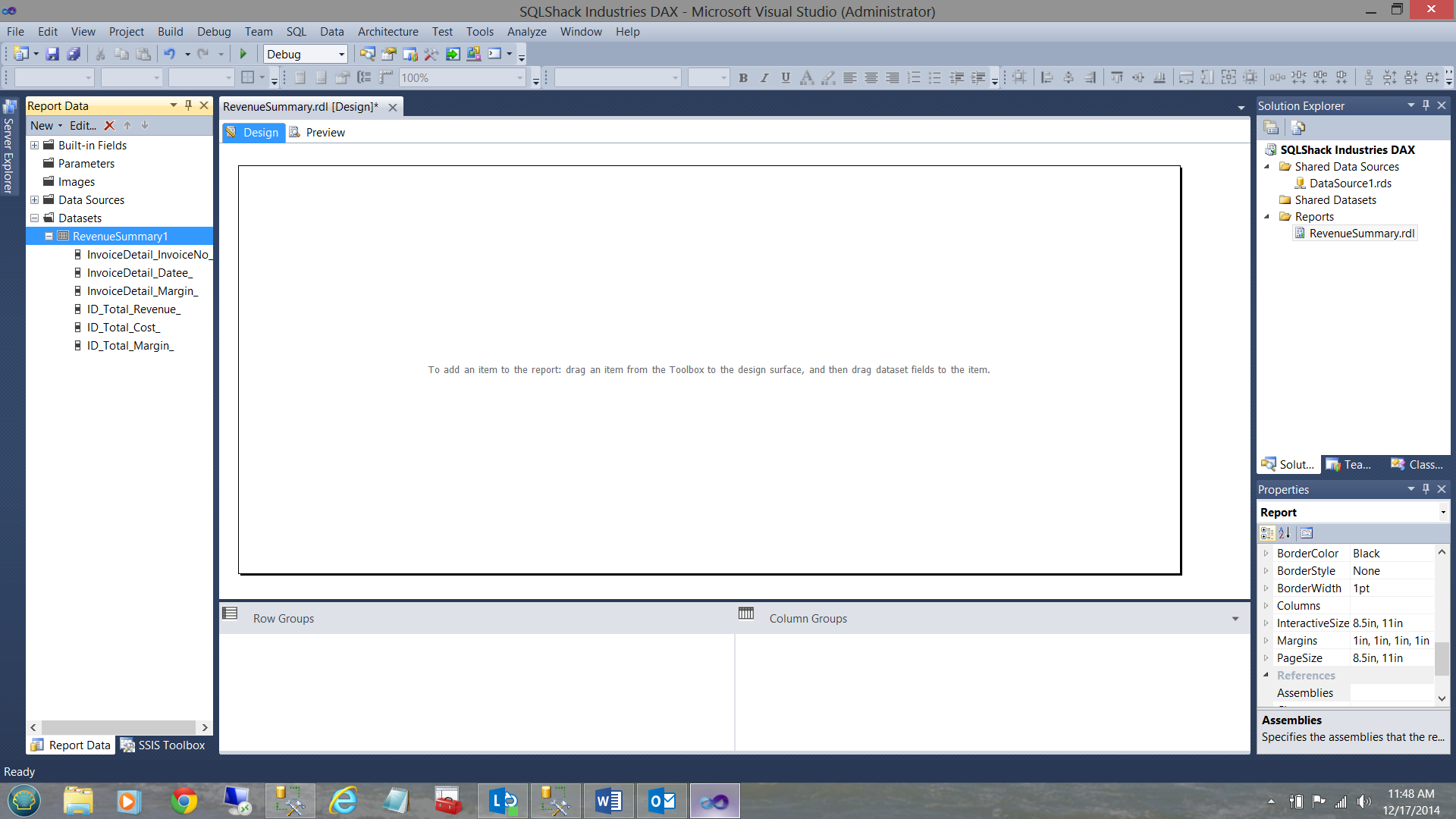
We now find ourselves back at the report “drawing surface”.
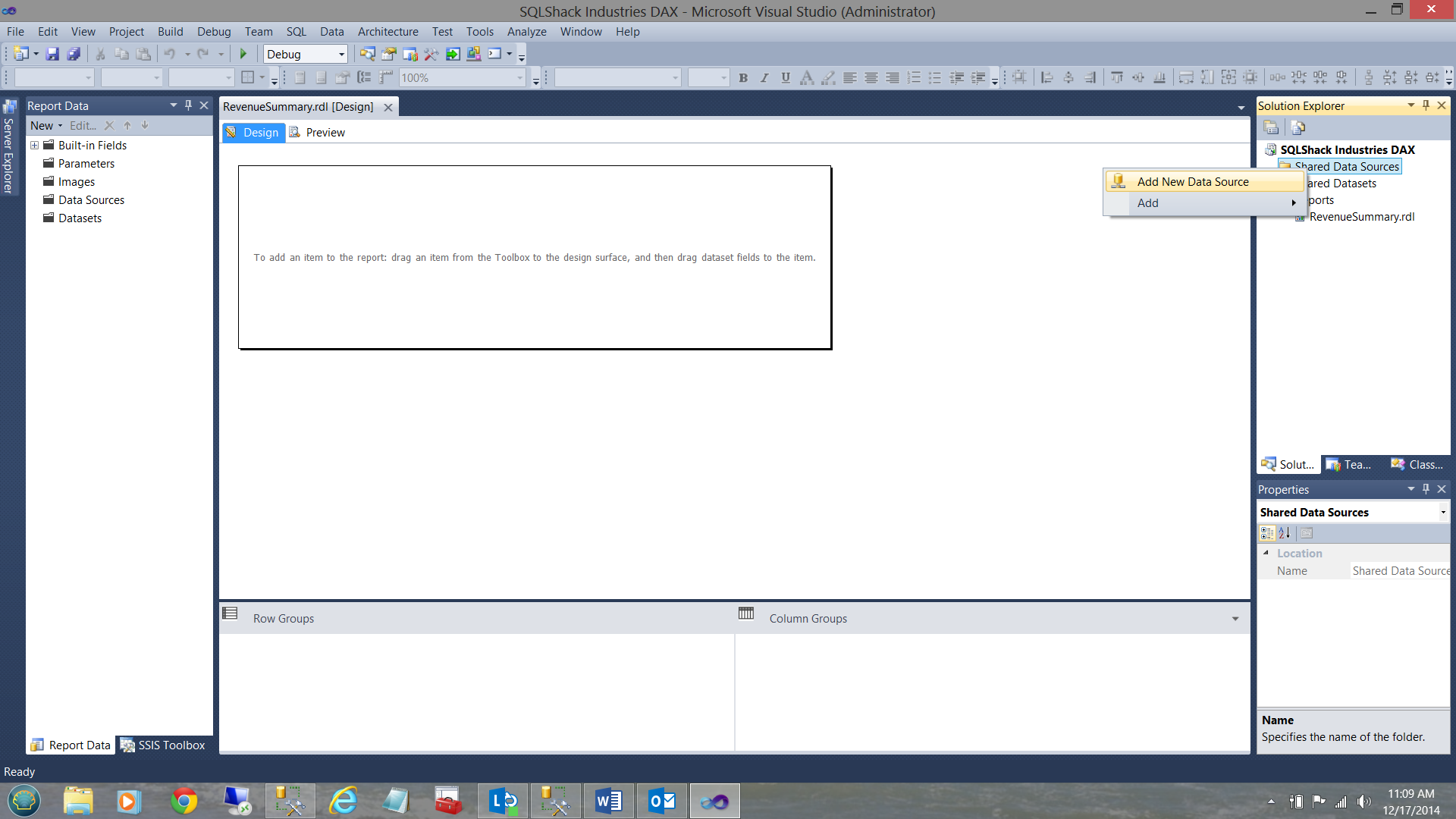
Our first task is to create a “Shared Data Source” (as we have in past articles).
I right click on the “Shared Data Source” folder and select “Add New Data Source”
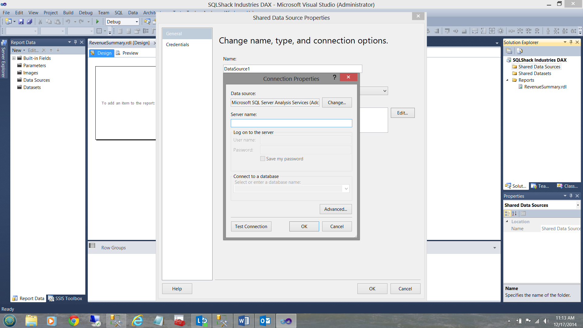
The “Shared Data Source” properties box is shown (see below).
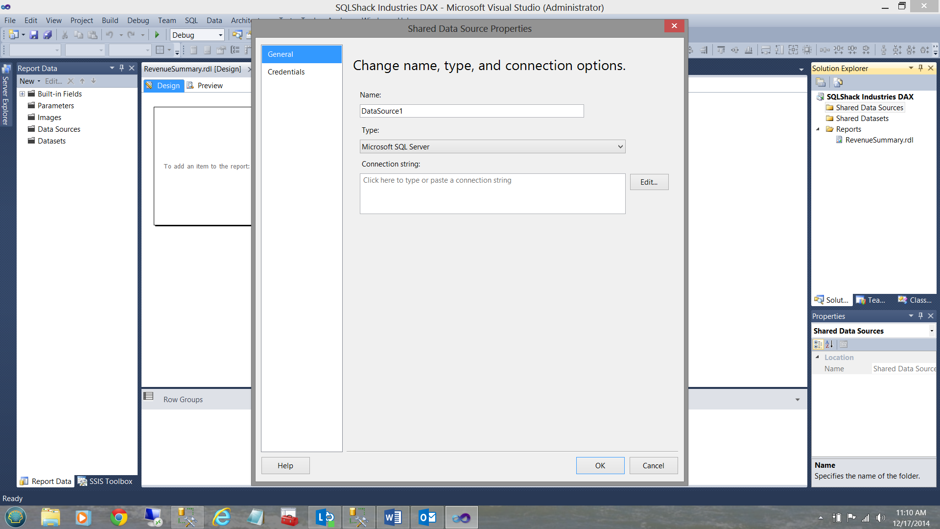
We CHANGE the “Type” box to “Microsoft SQL Server Analysis Services” (see below).

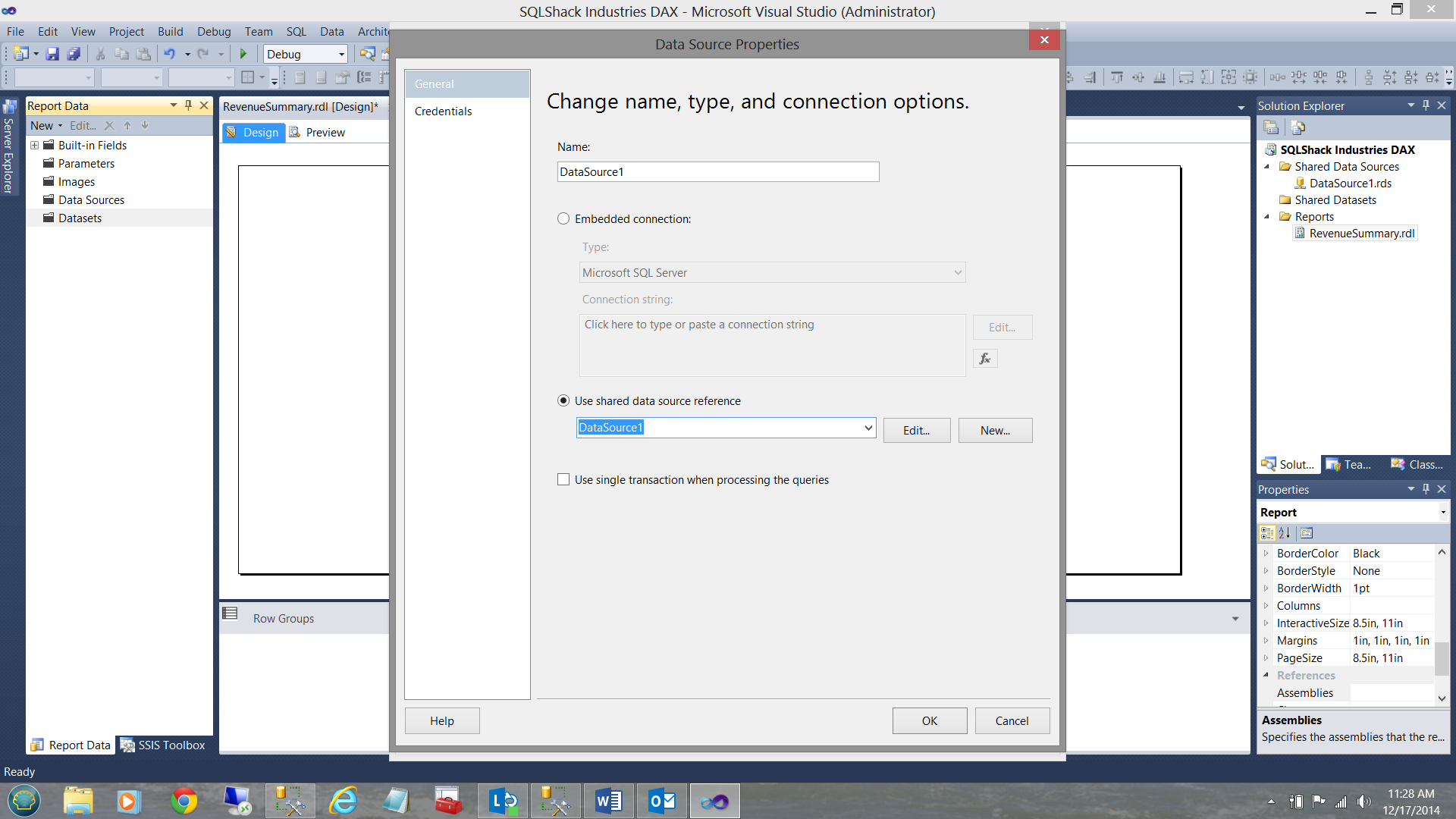
We now click the “Edit” button and the “Change name, type and connection options” dialog box is displayed (see below).
I now set my server and choose our “SalesCommissionReport” database and test the connection (see below).
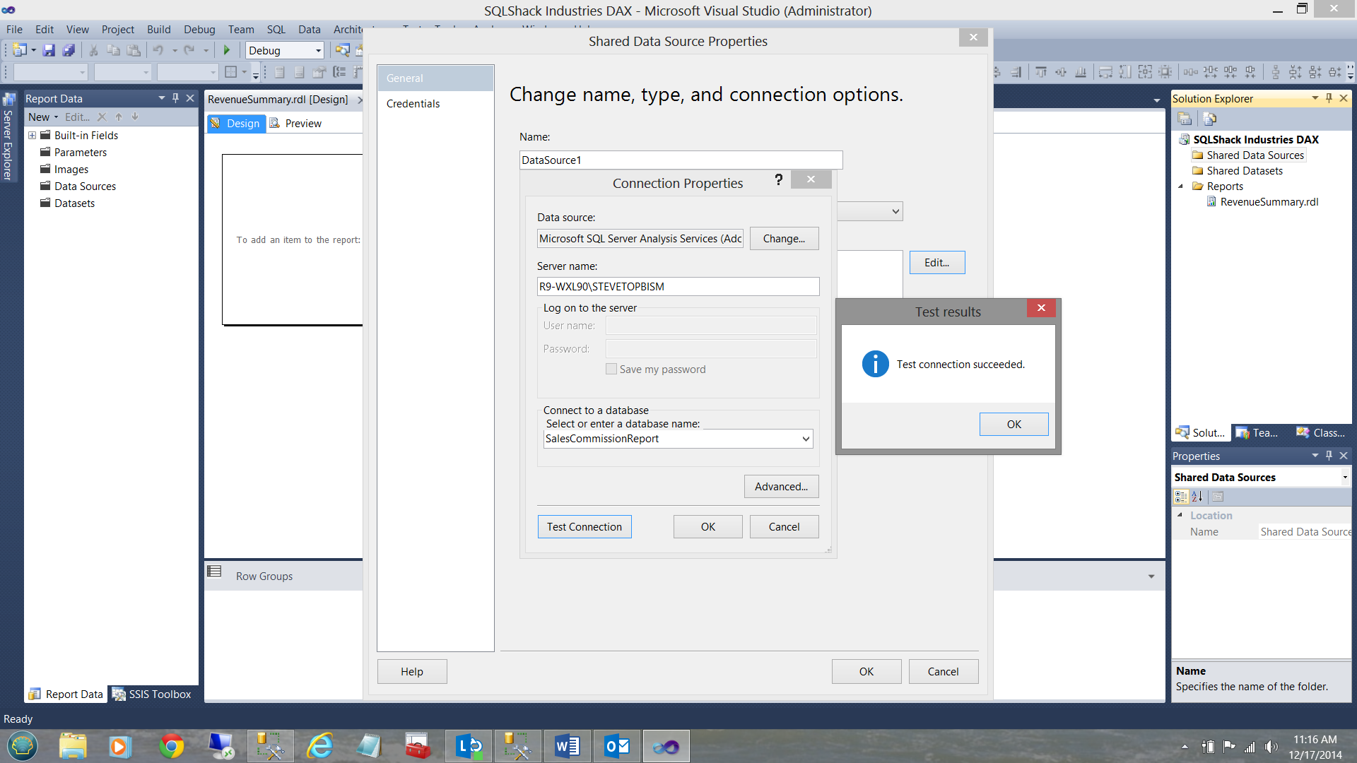
We click OK, OK and OK to exit and we are now ready to go!!
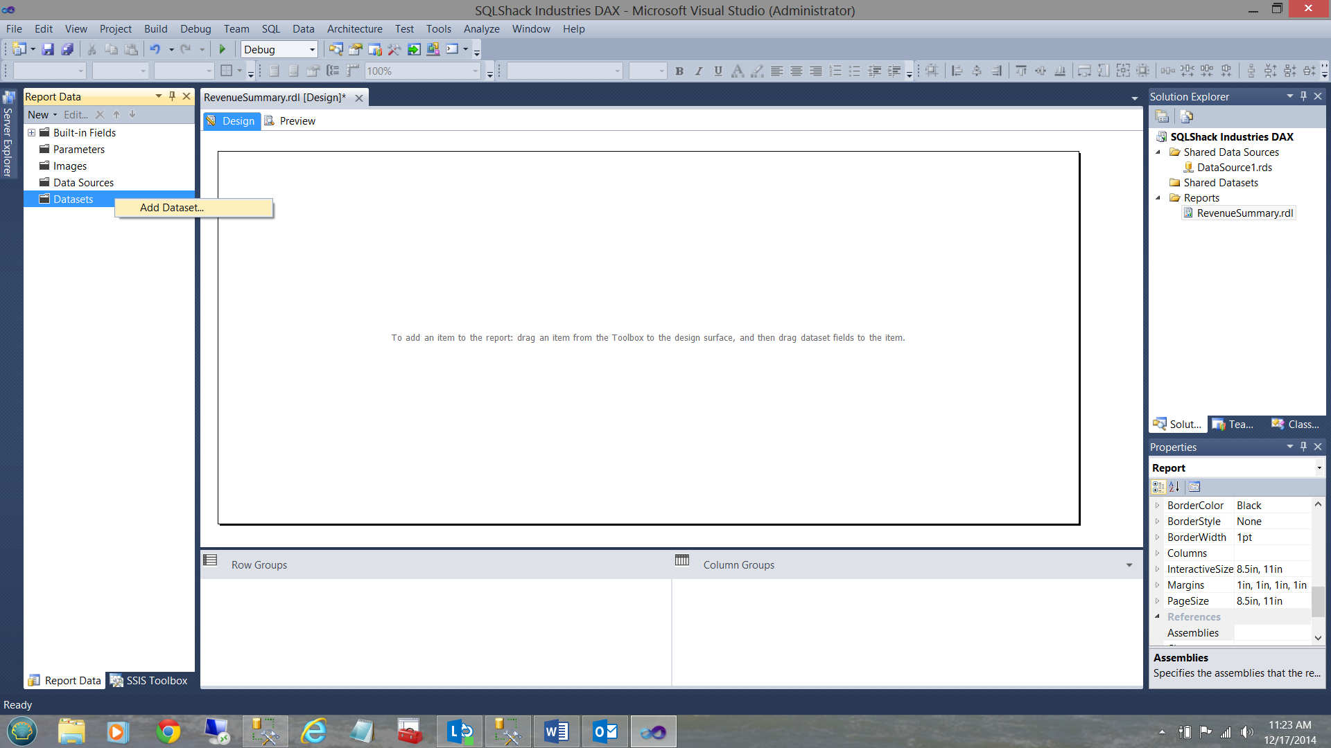
Once back on the drawing surface our first task is to create a data set to hold data PULLED from the Analysis Services tabular database. As I have described in earlier articles, a dataset may be likened to a bucket that is filled with water via a hose pipe coming from the faucet on the outside wall of your house. We then use the bucket of water to water the plants and in our case (with data) to populate our report(s).
AT THIS POINT I WOULD ASK THAT WE FOLLOW THE NEXT STEPS CAREFULLY as Microsoft has still to properly define a proper method to create TABULAR DATA sets. We MUST utilize a work-around.
We right click on the “Data Set” folder and select “Add Dataset”
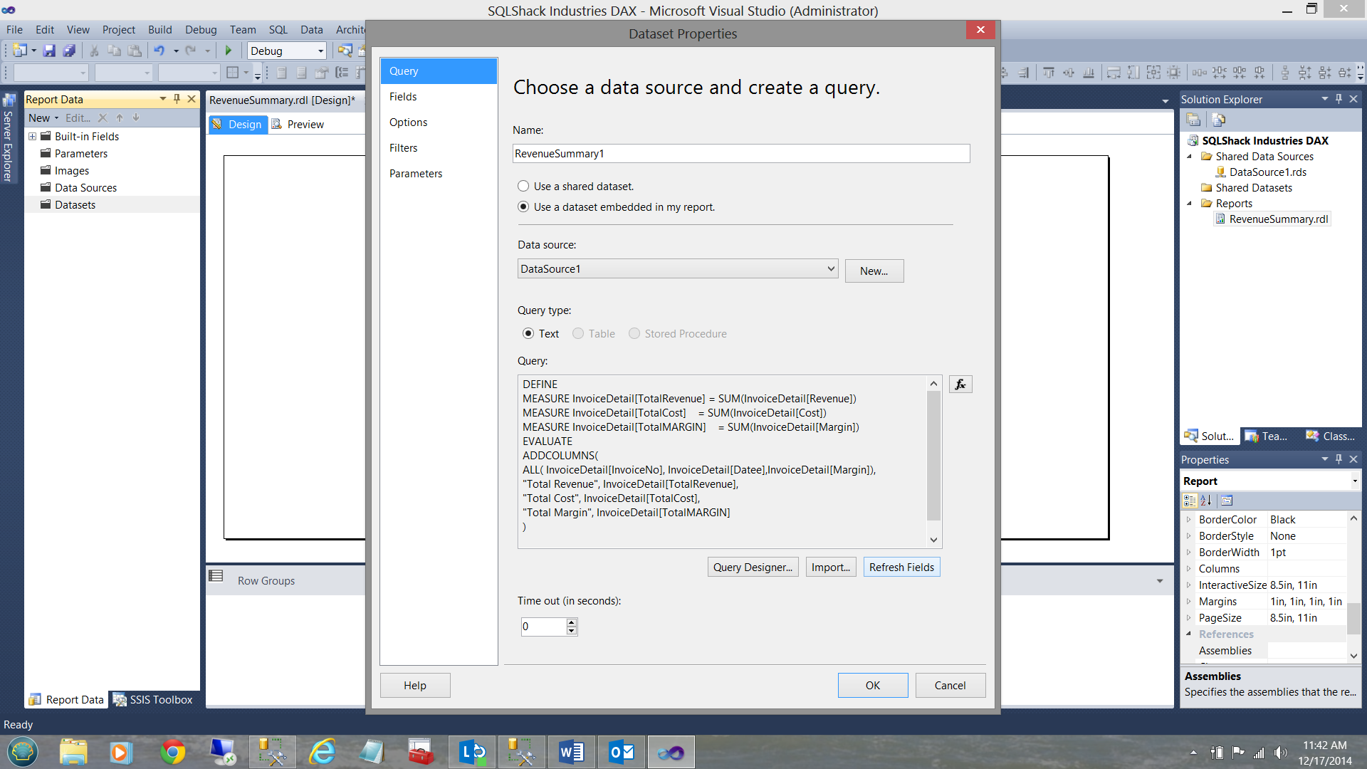
The “Choose a data source and create a query” dialog box appears (see below).
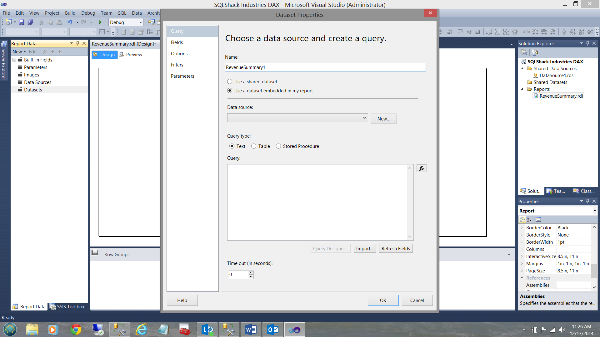
I give my dataset a name (see above) and click “New” to create a new local data source (for this report only) see above.
The “New data source” box is brought up and I select our share data source that we defined a few seconds ago (see below).
I click OK to exit the “Data Source” dialog. We find ourselves back at the “Data Set” dialog box.
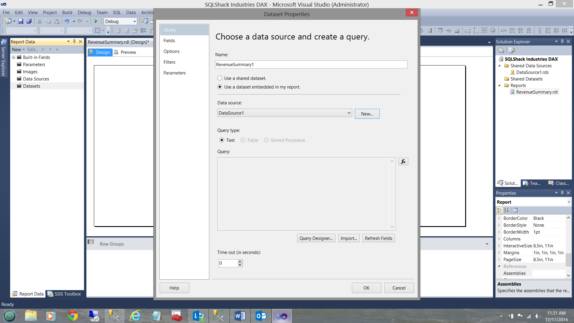
Now our queries are in fact text and the eagle-eyed reader will note that the “Query” dialog box is “greyed out”. Let the fun and games begin!!!
What is required to get Reporting Services to accept our DAX code is to select the “Query Designer” button (see above).
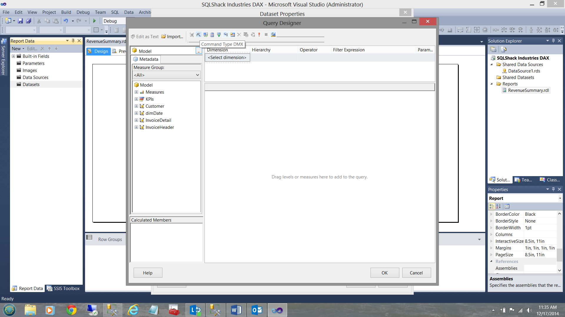
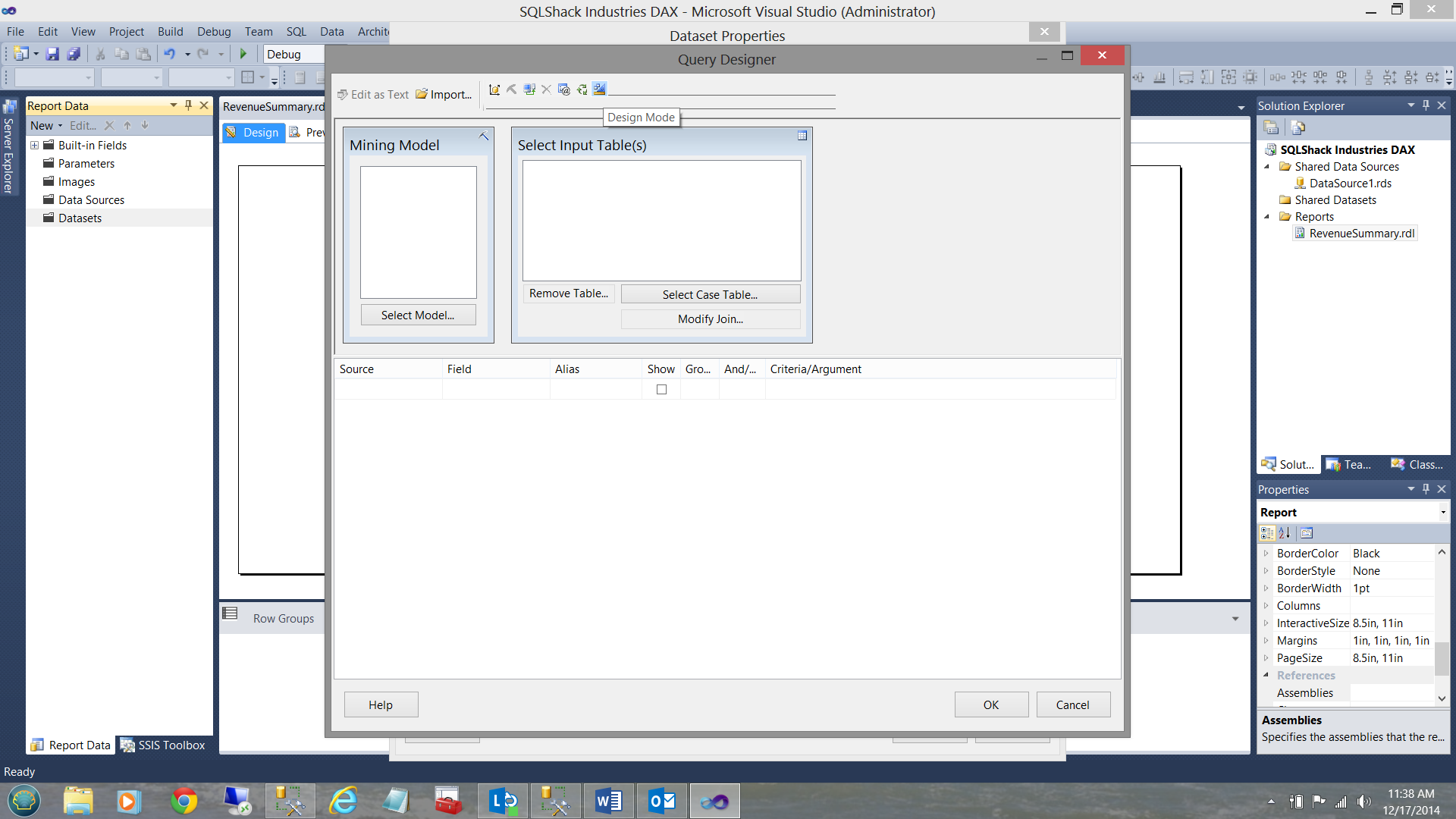
Clicking the “Query Designer” button brings up the “Query Designer” dialog box.
At this point we MUST SELECT “COMMAND TYPE DMX”. The button is found immediately above the “Command Type DMX” tool tip (see below).
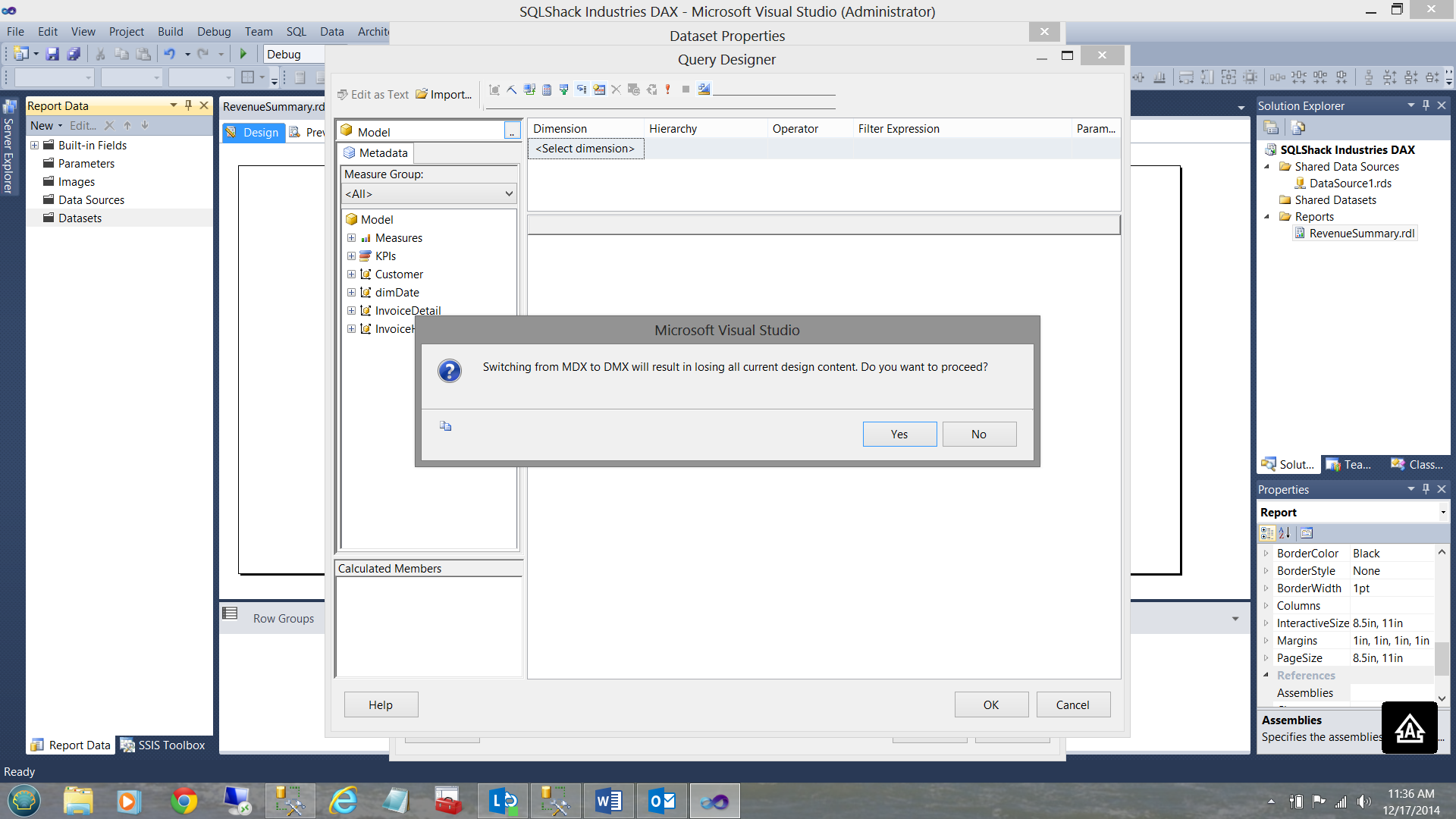
We are then informed that “Switching from MDX to DMX will result in losing all current design content. Do you want to proceed?” We click “Yes”.
We now choose to go into design mode (see below). The button is found immediately above the “Design Mode” tool tip (see below).
We are now finally able to insert our query (see below).
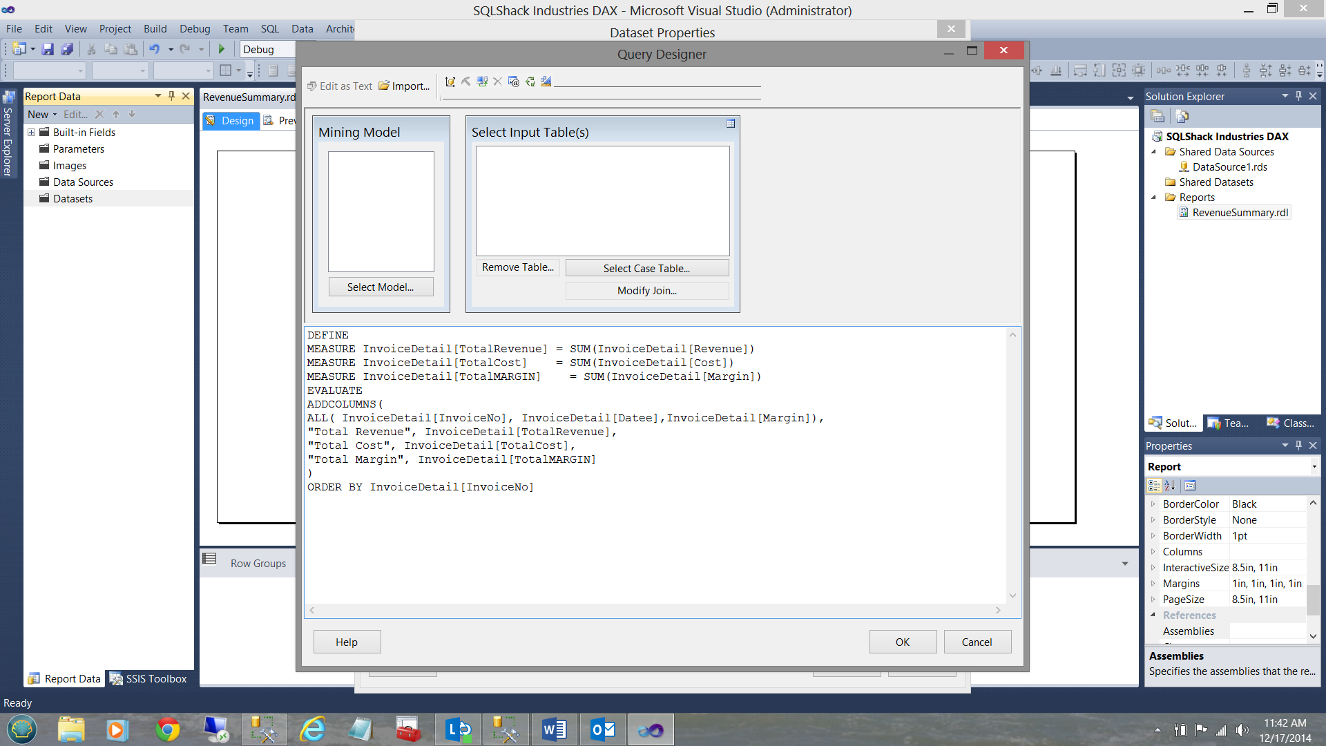
Click OK to complete the process.
We are returned to our create data set screen. We now click “Refresh Fields” in the lower right hand portion of the screen dump above. We now select the “Fields” tab in the upper left have portion of the screen dump below.
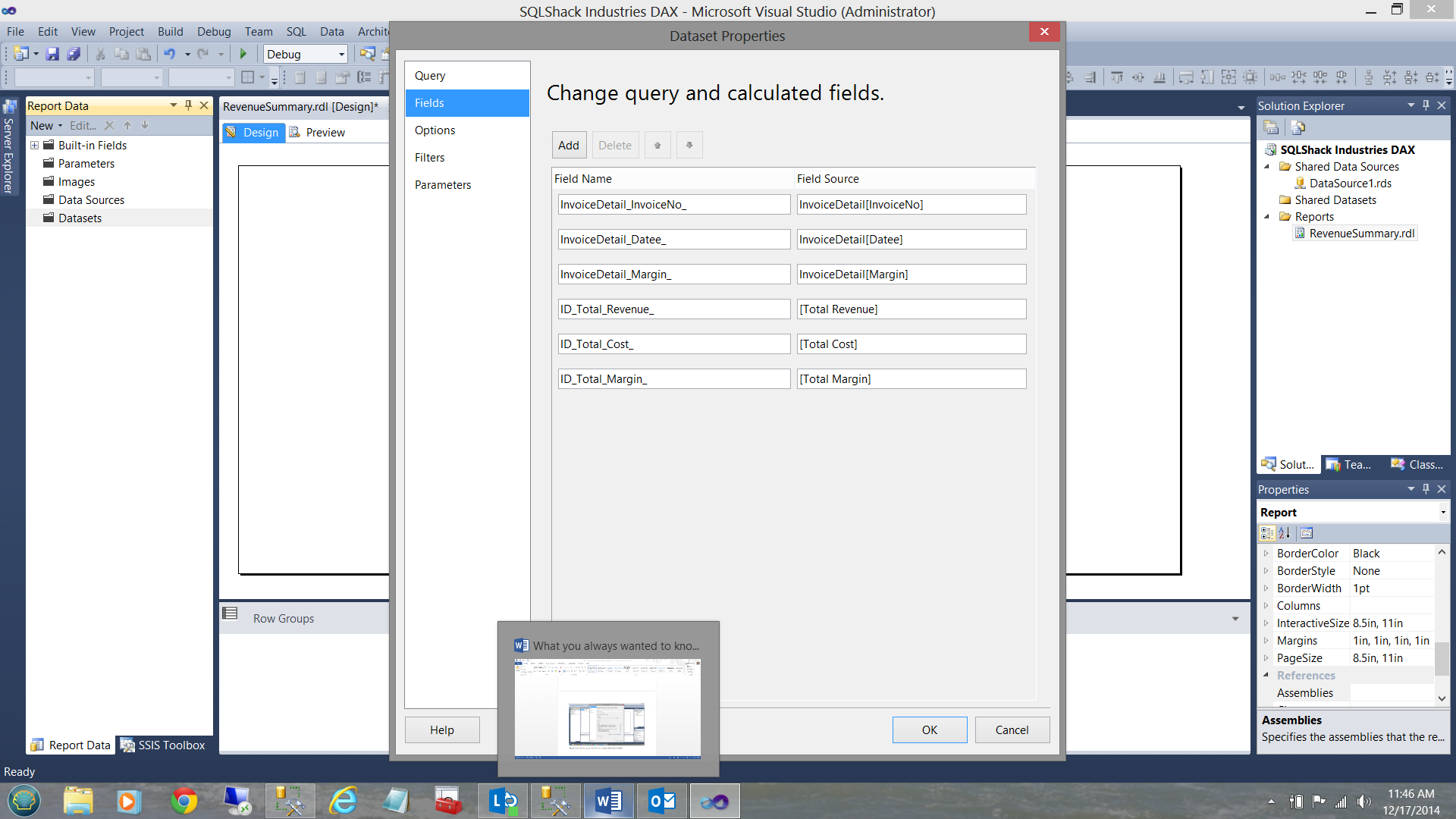
The fields for our query may be seen above. Click OK to leave the “Data Set” dialog.
We find ourselves back on the drawing surface with our data set created.
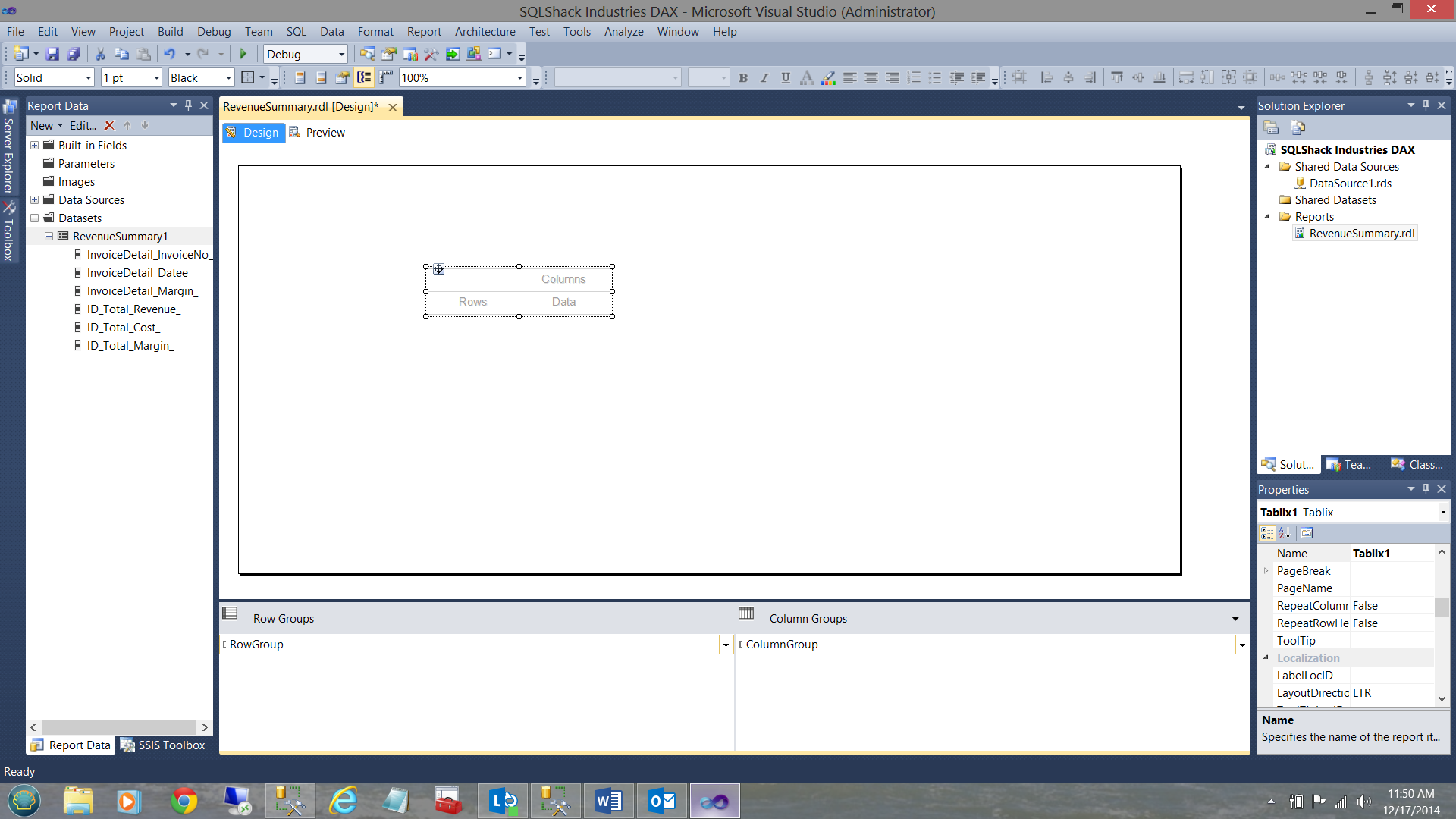
Next, we drag a “Matrix” onto the drawing surface (see below).
We now remove the “Column Groups” by right clicking on the [Column Group] and select removing grouping only (see below).
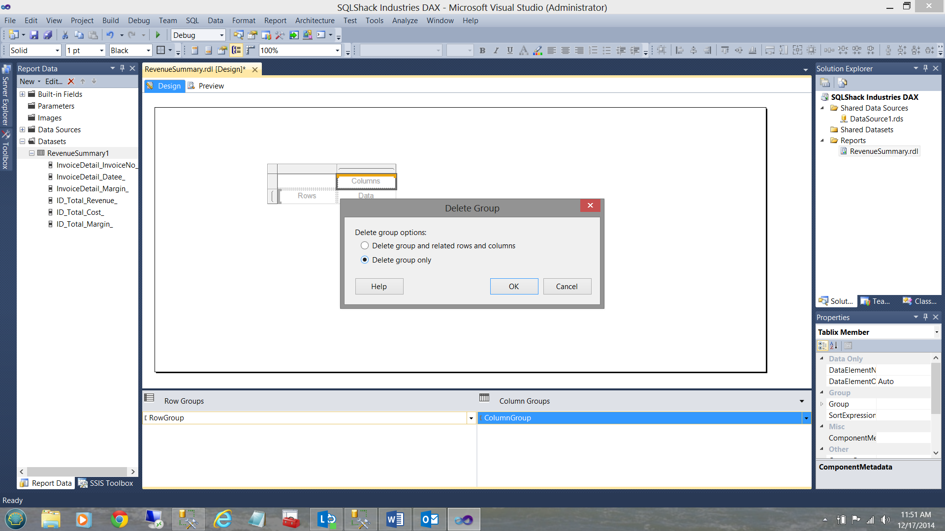
We click OK to accept and leave the “Delete Group” dialog.
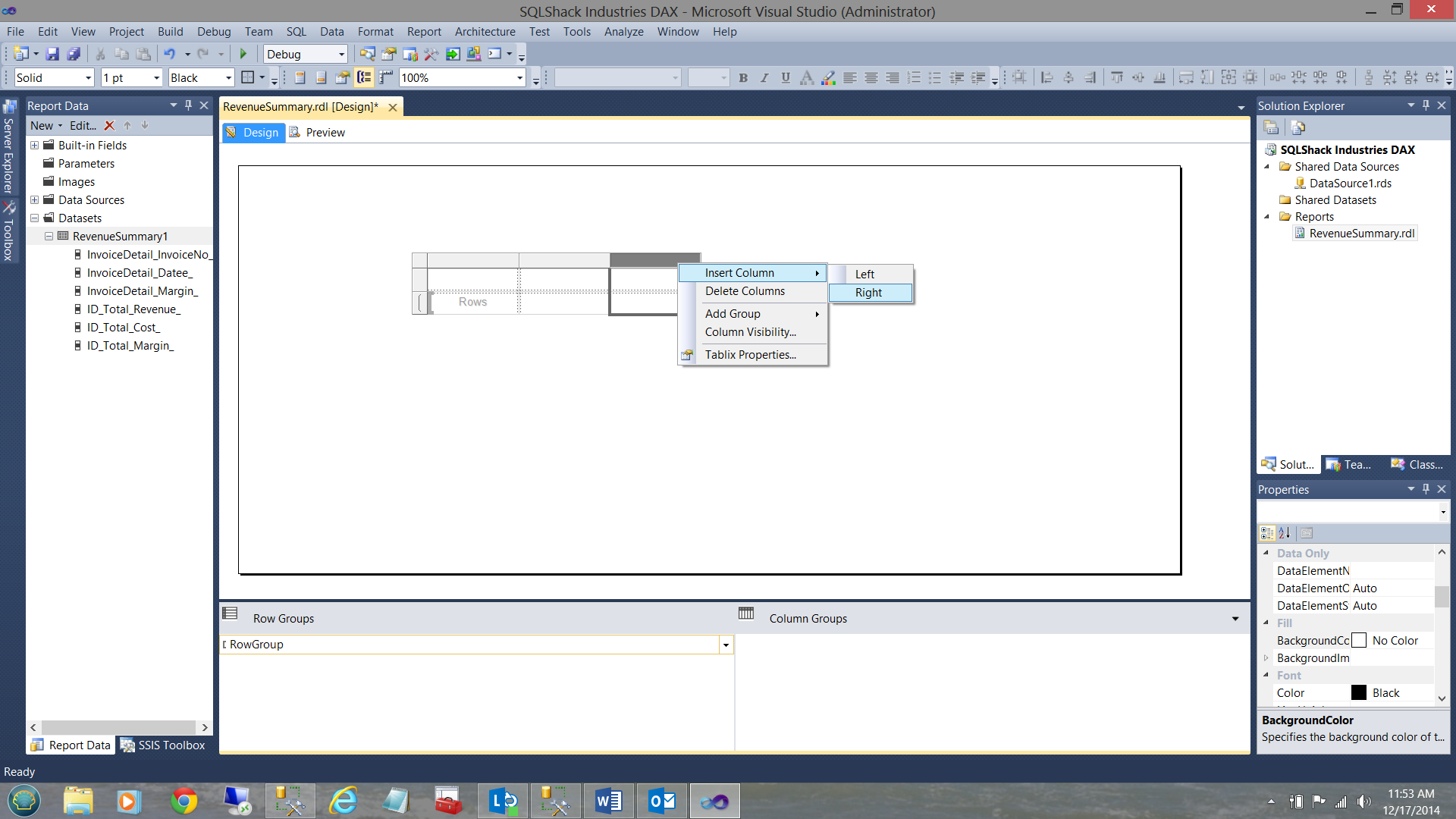
We now insert four more columns by right clicking on the top margin of the matrix (shown in black above).

Our finished surface may be seen above.
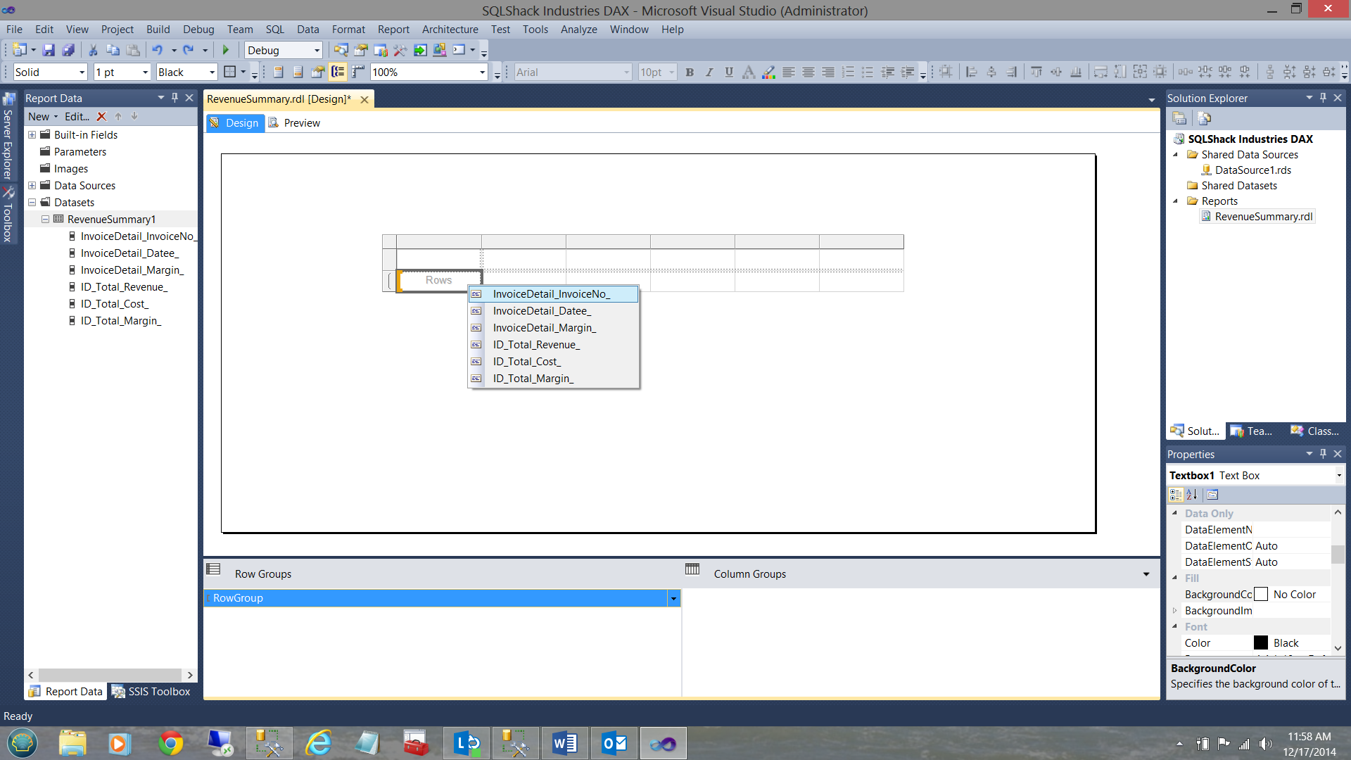
We now insert our first field (see above).
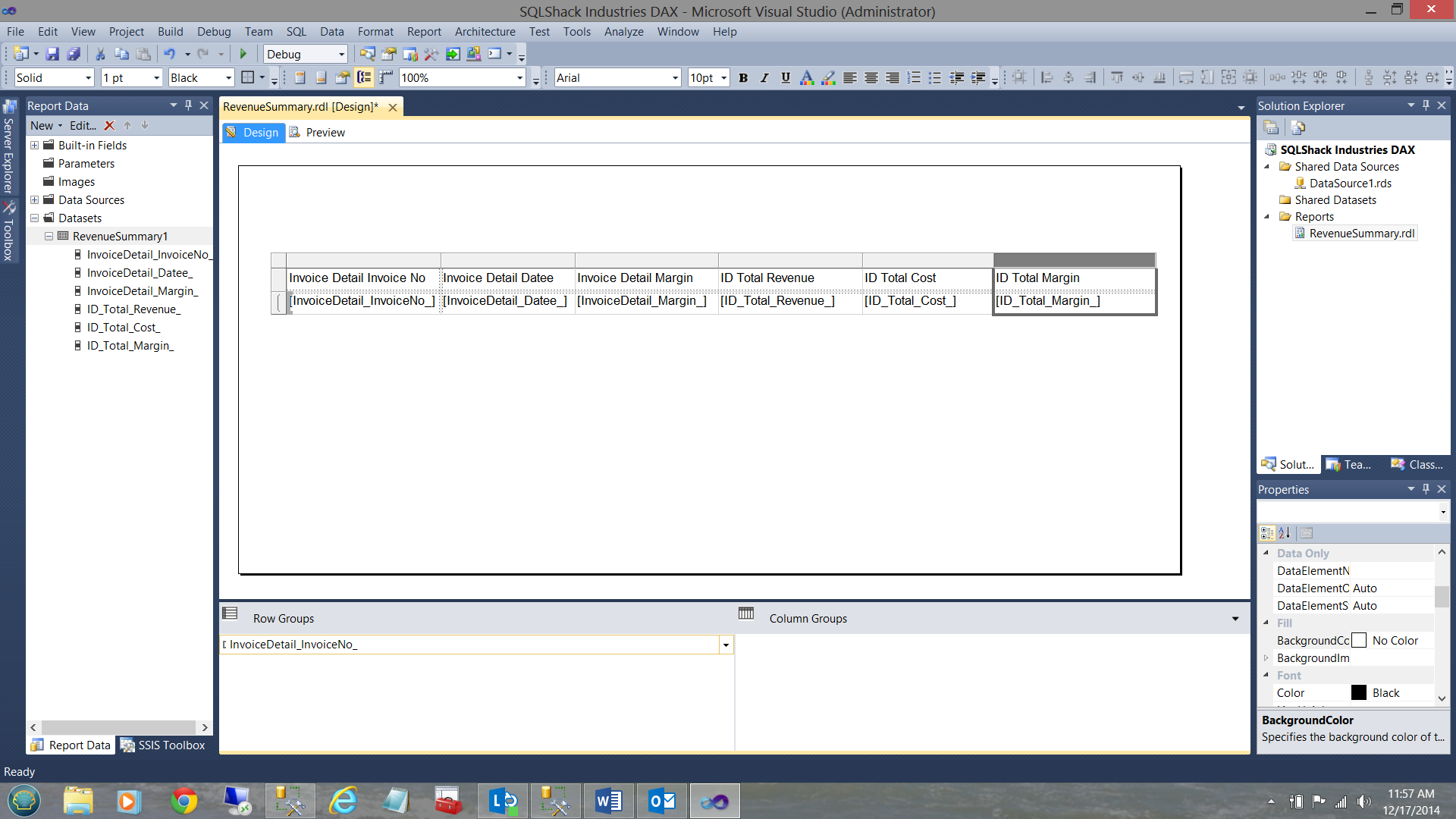
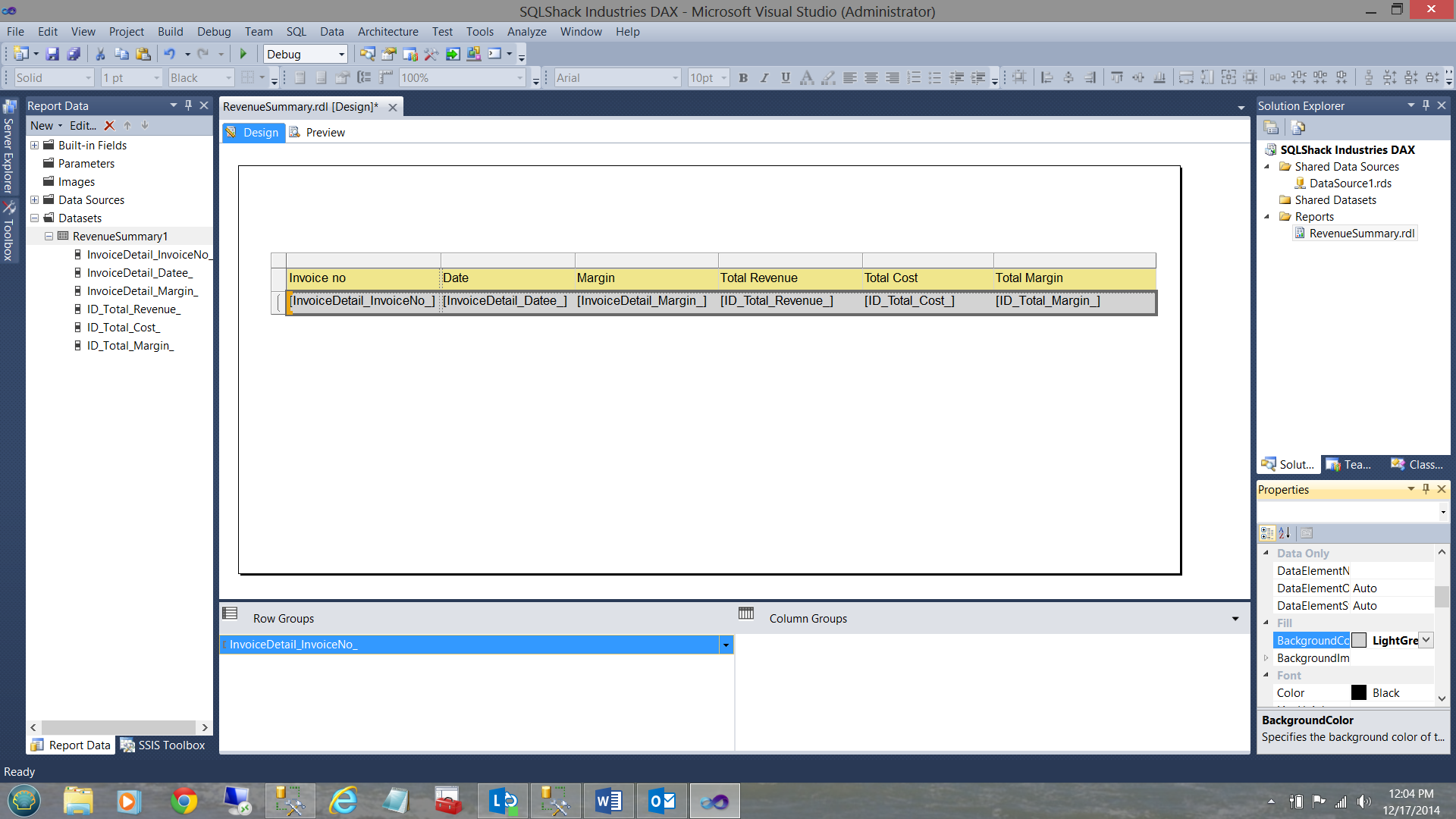
The screen shot above shows the matrix once all of the fields have been populated.
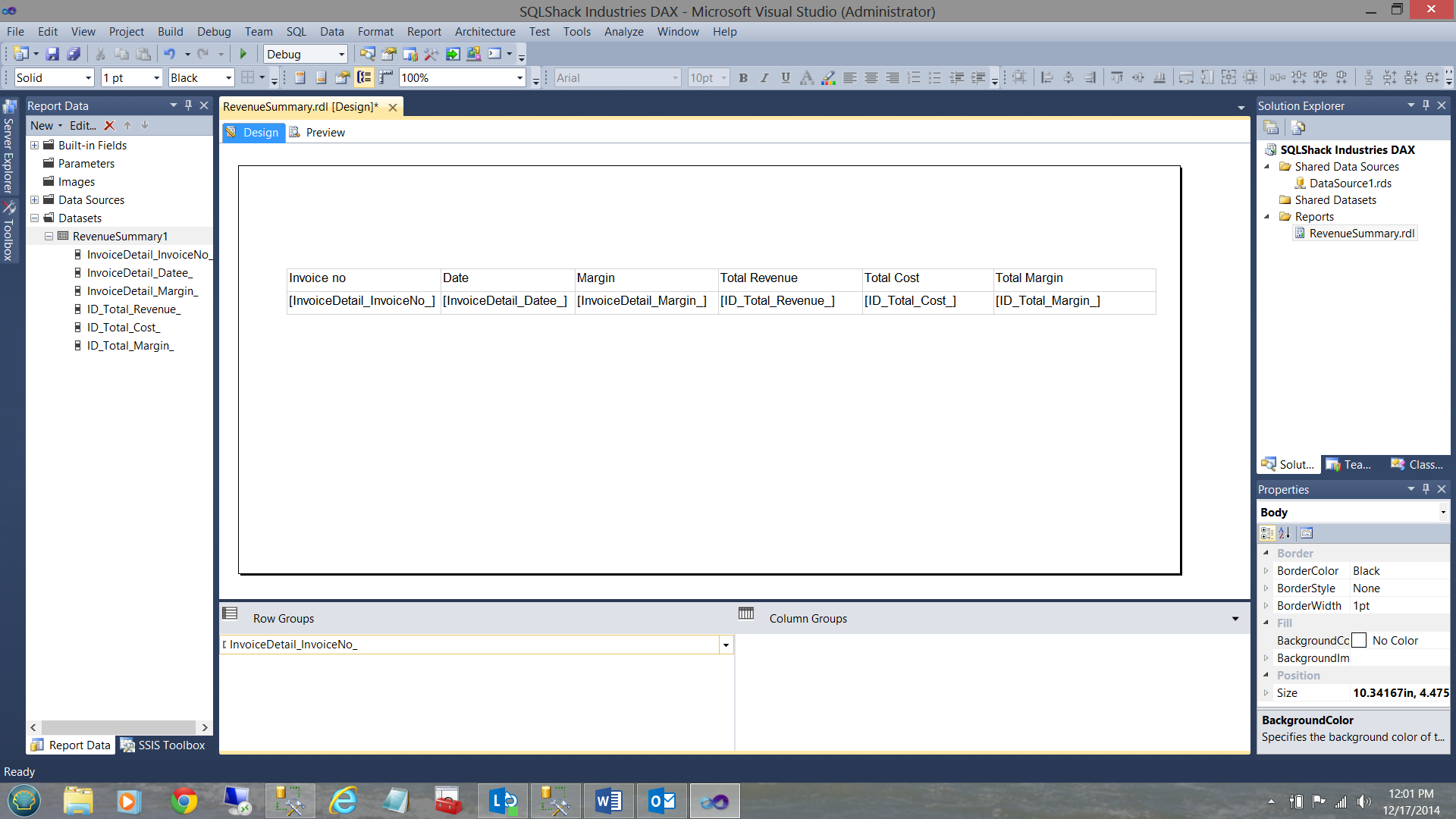
Looking at the column headings, we find them a bit cryptic. We shall change them as follows (see below).
Finally, we wish to change the ‘Hum Drum’ appearance by adding some fill to our text boxes. We choose “Khaki” for the headers and “Light Grey” for the values themselves.
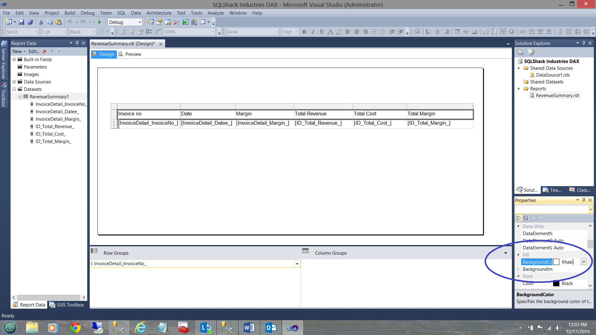
..and
The “value” or result text boxes are filled in with Light Grey.
Let us give our report a whirl by selecting “Preview”
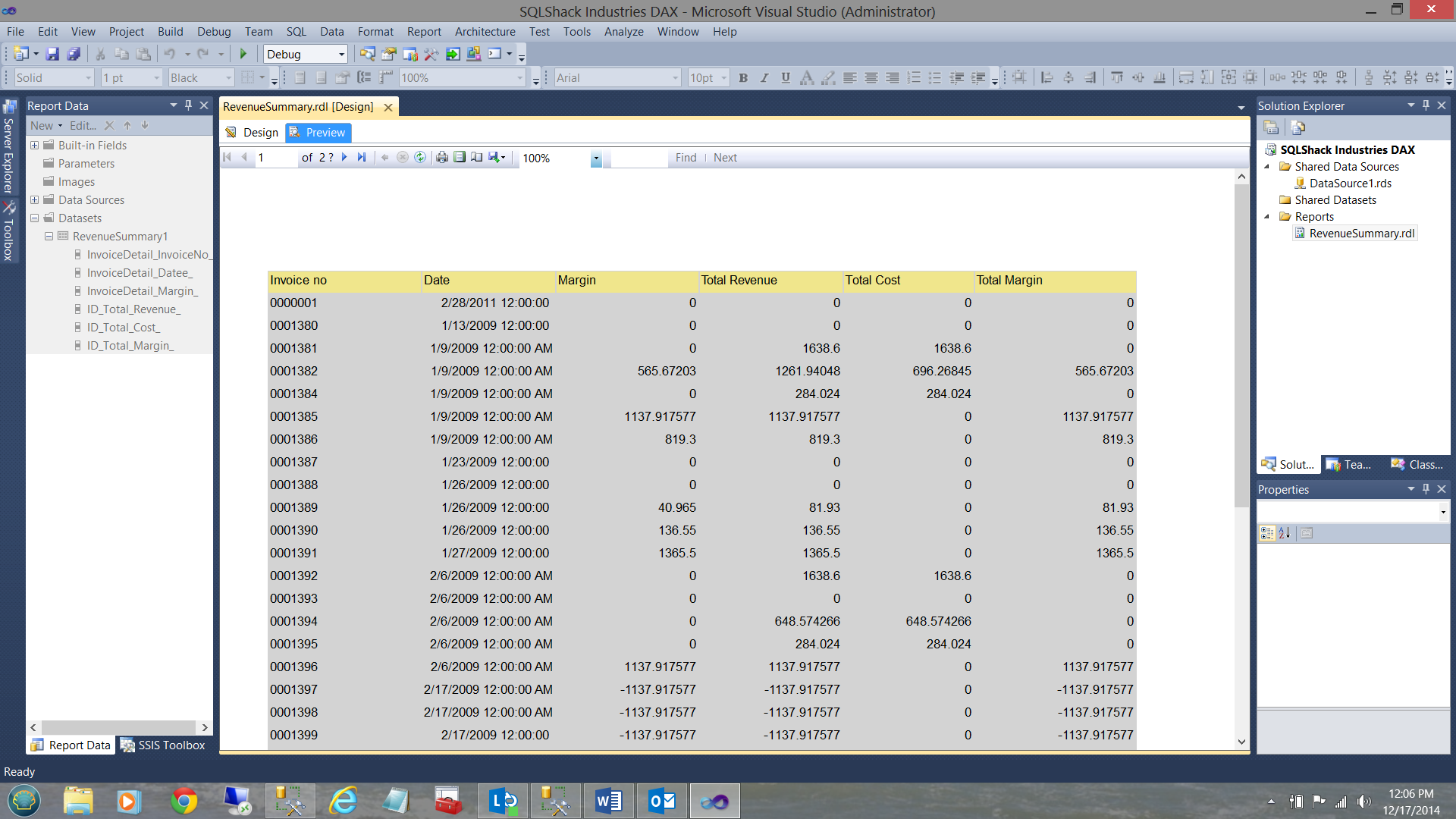
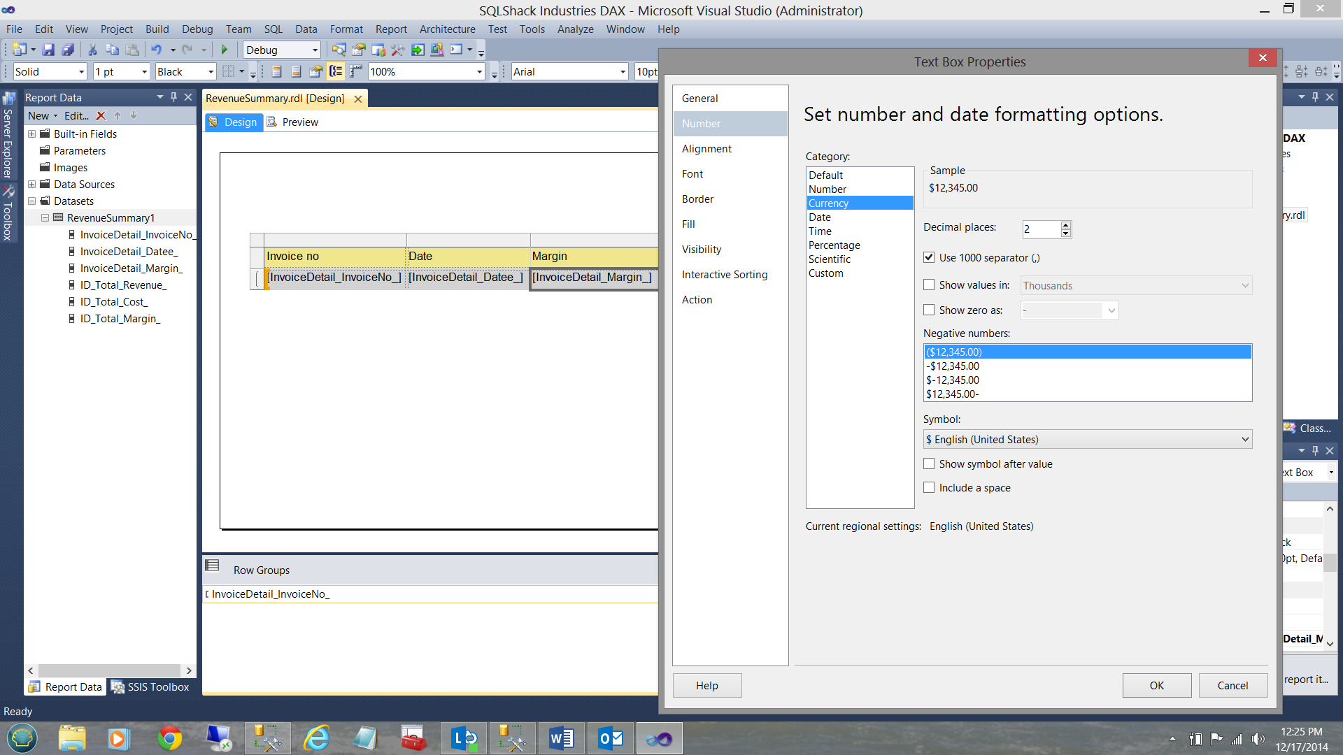
Here are the results. A mentioned earlier, we must now convert the date times to dates and have the dollar fields show only two decimal places.
We do so as follows:
Right clicking on the “datee” field “result box”, bring up the Textbox Properties dialog box (see below).
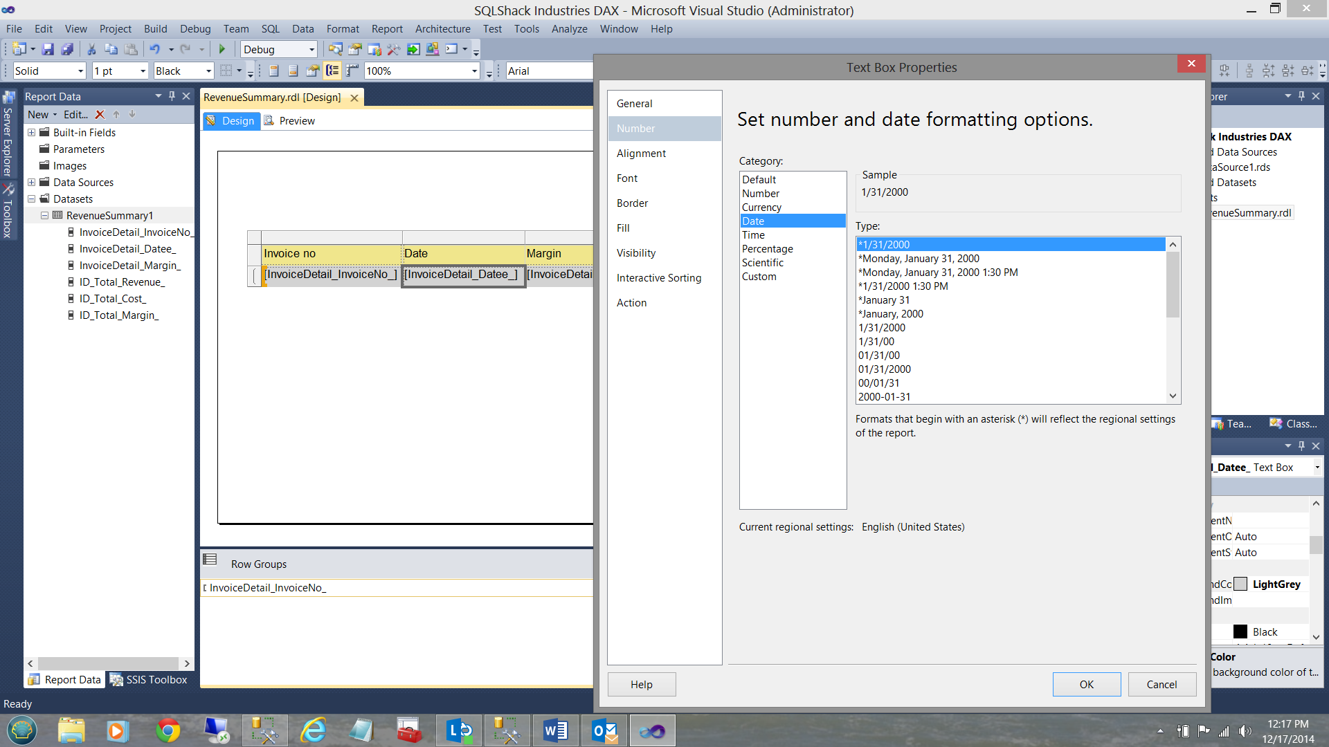
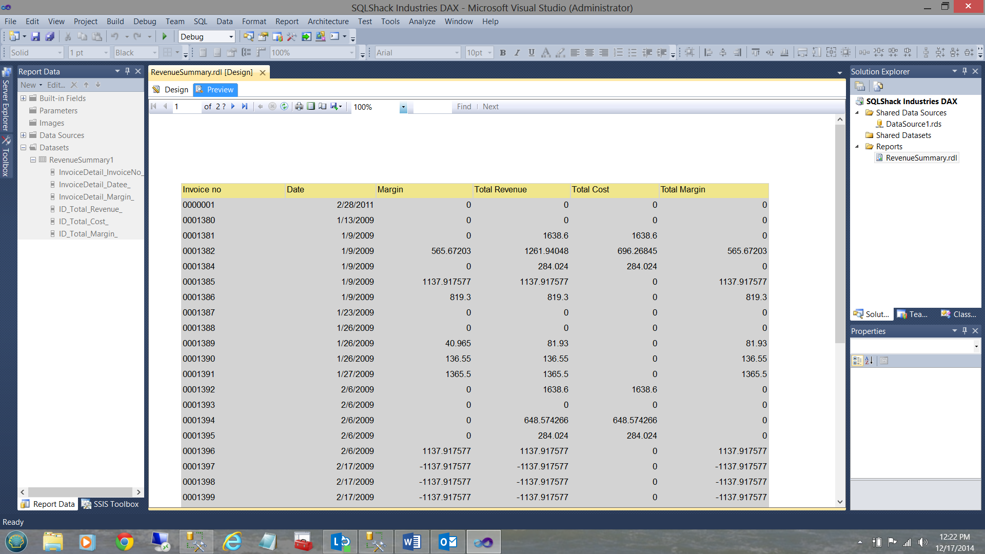
We select “Number”,”Date” and choose a format and click OK to finish. Our report now looks as follows.
Changing the “dollar” values, we now see the following:
And the final report…

Thus our report is complete and ready for the production environment!!!
Creating reports number two and three
I have taken the liberty of creating these two reports with the remaining two queries that we created above. The report creating process is the same as we have just seen for our Revenue Summary report.
And last but not least our “Same Period Last Year” report.
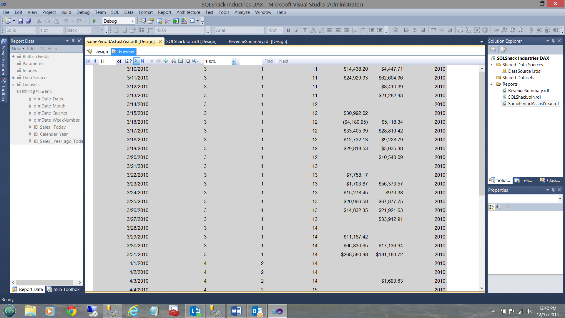
Thus we have completed our first venture into utilizing DAX expressions for queries which will be eventually utilized for reporting. Further they may be utilized with any data extracts utilizing Excel. But that is for another day.
Conclusions
With Power BI being the “Top of the pops” for reporting purposes within major industries and enterprises, it is and will become necessary for most SQL developers and BI specialists alike to become more fluent with the DAX language. More so for those enterprises that are heavily dependent on reporting via Excel.
Whilst DAX seems complex at first, it is fairly easy to learn and in doing so, you will put yourself ahead of the curve.
Happy programming!!!
Steve has presented papers at 8 PASS Summits and one at PASS Europe 2009 and 2010. He has recently presented a Master Data Services presentation at the PASS Amsterdam Rally.
Steve has presented 5 papers at the Information Builders' Summits. He is a PASS regional mentor.
View all posts by Steve Simon
- Reporting in SQL Server – Using calculated Expressions within reports - December 19, 2016
- How to use Expressions within SQL Server Reporting Services to create efficient reports - December 9, 2016
- How to use SQL Server Data Quality Services to ensure the correct aggregation of data - November 9, 2016