
All database users know about regular aggregate functions which operate on an entire table and are used with a GROUP BY clause. But very few people use Window functions in SQL. These operate on a set of rows and return a single aggregated value for each row.
The main advantage of using Window functions over regular aggregate functions is: Window functions do not cause rows to become grouped into a single output row, the rows retain their separate identities and an aggregated value will be added to each row.
Let’s take a look at how Window functions work and then see a few examples of using it in practice to be sure that things are clear and also how the SQL and output compare to that for SUM() functions.
As always be sure that you are fully backed up, especially if you are trying out new things with your database.
Introduction to Window functions
Window functions operate on a set of rows and return a single aggregated value for each row. The term Window describes the set of rows in the database on which the function will operate.
We define the Window (set of rows on which functions operates) using an OVER() clause. We will discuss more about the OVER() clause in the article below.
Types of Window functions
-
Aggregate Window Functions
SUM(), MAX(), MIN(), AVG(). COUNT() -
Ranking Window Functions
RANK(), DENSE_RANK(), ROW_NUMBER(), NTILE() -
Value Window Functions
LAG(), LEAD(), FIRST_VALUE(), LAST_VALUE()
Syntax
|
1 2 3 4 |
window_function ( [ ALL ] expression ) OVER ( [ PARTITION BY partition_list ] [ ORDER BY order_list] ) |
Arguments
window_function
Specify the name of the window function
ALL
ALL is an optional keyword. When you will include ALL it will count all values including duplicate ones. DISTINCT is not supported in window functions
expression
The target column or expression that the functions operates on. In other words, the name of the column for which we need an aggregated value. For example, a column containing order amount so that we can see total orders received.
OVER
Specifies the window clauses for aggregate functions.
PARTITION BY partition_list
Defines the window (set of rows on which window function operates) for window functions.
We need to provide a field or list of fields for the partition after PARTITION BY clause. Multiple fields need be separated by a comma as usual. If PARTITION BY is not specified, grouping will be done on entire table and values will be aggregated accordingly.
ORDER BY order_list
Sorts the rows within each partition. If ORDER BY is not specified, ORDER BY uses the entire table.
Examples
Let’s create table and insert dummy records to write further queries. Run below code.
|
1 2 3 4 5 6 7 8 9 10 11 12 13 14 15 16 17 18 19 20 21 22 23 24 25 26 27 28 29 30 31 |
CREATE TABLE [dbo].[Orders] ( order_id INT, order_date DATE, customer_name VARCHAR(250), city VARCHAR(100), order_amount MONEY ) INSERT INTO [dbo].[Orders] SELECT '1001','04/01/2017','David Smith','GuildFord',10000 UNION ALL SELECT '1002','04/02/2017','David Jones','Arlington',20000 UNION ALL SELECT '1003','04/03/2017','John Smith','Shalford',5000 UNION ALL SELECT '1004','04/04/2017','Michael Smith','GuildFord',15000 UNION ALL SELECT '1005','04/05/2017','David Williams','Shalford',7000 UNION ALL SELECT '1006','04/06/2017','Paum Smith','GuildFord',25000 UNION ALL SELECT '1007','04/10/2017','Andrew Smith','Arlington',15000 UNION ALL SELECT '1008','04/11/2017','David Brown','Arlington',2000 UNION ALL SELECT '1009','04/20/2017','Robert Smith','Shalford',1000 UNION ALL SELECT '1010','04/25/2017','Peter Smith','GuildFord',500 |
Aggregate Window Functions
SUM()
We all know the SUM() aggregate function. It does the sum of specified field for specified group (like city, state, country etc.) or for the entire table if group is not specified. We will see what will be the output of regular SUM() aggregate function and window SUM() aggregate function.
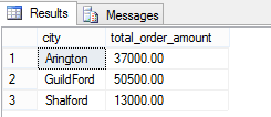
The following is an example of a regular SUM() aggregate function. It sums the order amount for each city.
You can see from the result set that a regular aggregate function groups multiple rows into a single output row, which causes individual rows to lose their identity.
|
1 2 3 4 |
SELECT city, SUM(order_amount) total_order_amount FROM [dbo].[Orders] GROUP BY city |
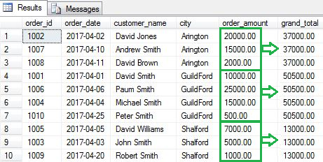
This does not happen with window aggregate functions. Rows retain their identity and also show an aggregated value for each row. In the example below the query does the same thing, namely it aggregates the data for each city and shows the sum of total order amount for each of them. However, the query now inserts another column for the total order amount so that each row retains its identity. The column marked grand_total is the new column in the example below.
|
1 2 3 4 5 |
SELECT order_id, order_date, customer_name, city, order_amount ,SUM(order_amount) OVER(PARTITION BY city) as grand_total FROM [dbo].[Orders] |
AVG()
AVG or Average works in exactly the same way with a Window function.
The following query will give you average order amount for each city and for each month (although for simplicity we’ve only used data in one month).
We specify more than one average by specifying multiple fields in the partition list.
It is also worth noting that that you can use expressions in the lists like MONTH(order_date) as shown in below query. As ever you can make these expressions as complex as you want so long as the syntax is correct!
|
1 2 3 4 5 |
SELECT order_id, order_date, customer_name, city, order_amount ,AVG(order_amount) OVER(PARTITION BY city, MONTH(order_date)) as average_order_amount FROM [dbo].[Orders] |
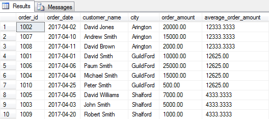
From the above image, we can clearly see that on an average we have received orders of 12,333 for Arlington city for April, 2017.
Average Order Amount = Total Order Amount / Total Orders
= (20,000 + 15,000 + 2,000) / 3
= 12,333
You can also use the combination of SUM() & COUNT() function to calculate an average.
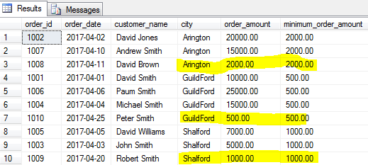
MIN()
The MIN() aggregate function will find the minimum value for a specified group or for the entire table if group is not specified.
For example, we are looking for the smallest order (minimum order) for each city we would use the following query.
|
1 2 3 4 5 |
SELECT order_id, order_date, customer_name, city, order_amount ,MIN(order_amount) OVER(PARTITION BY city) as minimum_order_amount FROM [dbo].[Orders] |
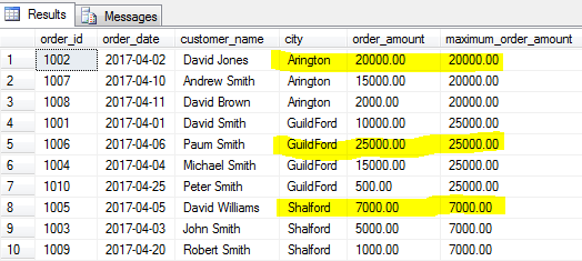
MAX()
Just as the MIN() functions gives you the minimum value, the MAX() function will identify the largest value of a specified field for a specified group of rows or for the entire table if a group is not specified.
let’s find the biggest order (maximum order amount) for each city.
|
1 2 3 4 5 |
SELECT order_id, order_date, customer_name, city, order_amount ,MAX(order_amount) OVER(PARTITION BY city) as maximum_order_amount FROM [dbo].[Orders] |
COUNT()
The COUNT() function will count the records / rows.
Note that DISTINCT is not supported with window COUNT() function whereas it is supported for the regular COUNT() function. DISTINCT helps you to find the distinct values of a specified field.
For example, if we want to see how many customers have placed an order in April 2017, we cannot directly count all customers. It is possible that the same customer has placed multiple orders in the same month.
COUNT(customer_name) will give you an incorrect result as it will count duplicates. Whereas COUNT(DISTINCT customer_name) will give you the correct result as it counts each unique customer only once.
Valid for regular COUNT() function:
|
1 2 3 4 5 |
SELECT city,COUNT(DISTINCT customer_name) number_of_customers FROM [dbo].[Orders] GROUP BY city |
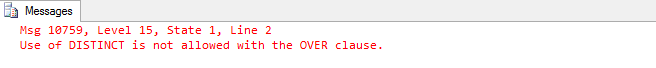
Invalid for window COUNT() function:
|
1 2 3 4 5 |
SELECT order_id, order_date, customer_name, city, order_amount ,COUNT(DISTINCT customer_name) OVER(PARTITION BY city) as number_of_customers FROM [dbo].[Orders] |
The above query with Window function will give you below error.
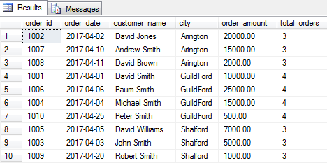
Now, let’s find the total order received for each city using window COUNT() function.
|
1 2 3 4 5 |
SELECT order_id, order_date, customer_name, city, order_amount ,COUNT(order_id) OVER(PARTITION BY city) as total_orders FROM [dbo].[Orders] |
Ranking Window Functions
Just as Window aggregate functions aggregate the value of a specified field, RANKING functions will rank the values of a specified field and categorize them according to their rank.
The most common use of RANKING functions is to find the top (N) records based on a certain value. For example, Top 10 highest paid employees, Top 10 ranked students, Top 50 largest orders etc.
The following are supported RANKING functions:
RANK(), DENSE_RANK(), ROW_NUMBER(), NTILE()Let’s discuss them one by one.
RANK()
The RANK() function is used to give a unique rank to each record based on a specified value, for example salary, order amount etc.
If two records have the same value then the RANK() function will assign the same rank to both records by skipping the next rank. This means – if there are two identical values at rank 2, it will assign the same rank 2 to both records and then skip rank 3 and assign rank 4 to the next record.
Let’s rank each order by their order amount.
|
1 2 3 4 5 |
SELECT order_id,order_date,customer_name,city, RANK() OVER(ORDER BY order_amount DESC) [Rank] FROM [dbo].[Orders] |
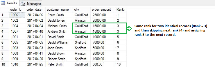
From the above image, you can see that the same rank (3) is assigned to two identical records (each having an order amount of 15,000) and it then skips the next rank (4) and assign rank 5 to next record.
DENSE_RANK()
The DENSE_RANK() function is identical to the RANK() function except that it does not skip any rank. This means that if two identical records are found then DENSE_RANK() will assign the same rank to both records but not skip then skip the next rank.
Let’s see how this works in practice.
|
1 2 3 4 5 |
SELECT order_id,order_date,customer_name,city, order_amount, DENSE_RANK() OVER(ORDER BY order_amount DESC) [Rank] FROM [dbo].[Orders] |
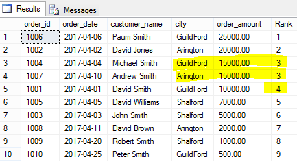
As you can clearly see above, the same rank is given to two identical records (each having the same order amount) and then the next rank number is given to the next record without skipping a rank value.
ROW_NUMBER()
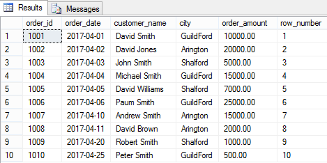
The name is self-explanatory. These functions assign a unique row number to each record.
The row number will be reset for each partition if PARTITION BY is specified. Let’s see how ROW_NUMBER() works without PARTITION BY and then with PARTITION BY.
ROW_ NUMBER() without PARTITION BY
|
1 2 3 4 5 |
SELECT order_id,order_date,customer_name,city, order_amount, ROW_NUMBER() OVER(ORDER BY order_id) [row_number] FROM [dbo].[Orders] |
ROW_NUMBER() with PARTITION BY
|
1 2 3 4 5 |
SELECT order_id,order_date,customer_name,city, order_amount, ROW_NUMBER() OVER(PARTITION BY city ORDER BY order_amount DESC) [row_number] FROM [dbo].[Orders] |
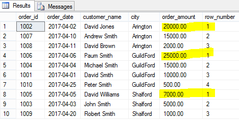
Note that we have done the partition on city. This means that the row number is reset for each city and so restarts at 1 again. However, the order of the rows is determined by order amount so that for any given city the largest order amount will be the first row and so assigned row number 1.
NTILE()
NTILE() is a very helpful window function. It helps you to identify what percentile (or quartile, or any other subdivision) a given row falls into.
This means that if you have 100 rows and you want to create 4 quartiles based on a specified value field you can do so easily and see how many rows fall into each quartile.
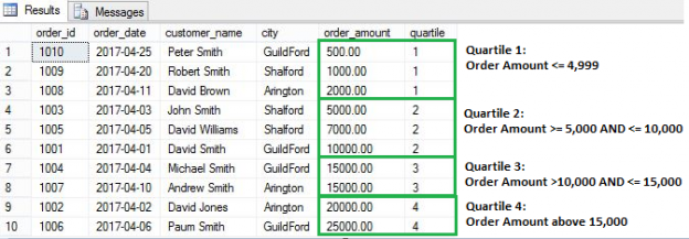
Let’s see an example. In the query below, we have specified that we want to create four quartiles based on order amount. We then want to see how many orders fall into each quartile.
|
1 2 3 4 5 |
SELECT order_id,order_date,customer_name,city, order_amount, NTILE(4) OVER(ORDER BY order_amount) [row_number] FROM [dbo].[Orders] |
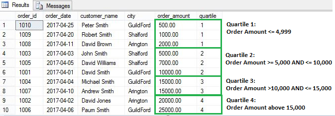
NTILE creates tiles based on following formula:
No of rows in each tile = number of rows in result set / number of tiles specified
Here is our example, we have total 10 rows and 4 tiles are specified in the query so number of rows in each tile will be 2.5 (10/4). As number of rows should be whole number, not a decimal. SQL engine will assign 3 rows for first two groups and 2 rows for remaining two groups.
Value Window Functions
Value window functions are used to find first, last, previous and next values. The functions that can be used are LAG(), LEAD(), FIRST_VALUE(), LAST_VALUE()
LAG() and LEAD()
LEAD() and LAG() functions are very powerful but can be complex to explain.
As this is an introductory article below we are looking at a very simple example to illustrate how to use them.
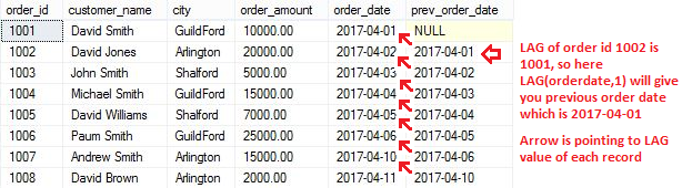
The LAG function allows to access data from the previous row in the same result set without use of any SQL joins. You can see in below example, using LAG function we found previous order date.
Script to find previous order date using LAG() function:
|
1 2 3 4 5 6 |
SELECT order_id,customer_name,city, order_amount,order_date, --in below line, 1 indicates check for previous row of the current row LAG(order_date,1) OVER(ORDER BY order_date) prev_order_date FROM [dbo].[Orders] |
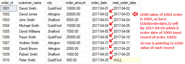
LEAD function allows to access data from the next row in the same result set without use of any SQL joins. You can see in below example, using LEAD function we found next order date.
Script to find next order date using LEAD() function:
|
1 2 3 4 5 6 |
SELECT order_id,customer_name,city, order_amount,order_date, --in below line, 1 indicates check for next row of the current row LEAD(order_date,1) OVER(ORDER BY order_date) next_order_date FROM [dbo].[Orders] |
FIRST_VALUE() and LAST_VALUE()
These functions help you to identify first and last record within a partition or entire table if PARTITION BY is not specified.
Let’s find the first and last order of each city from our existing dataset. Note ORDER BY clause is mandatory for FIRST_VALUE() and LAST_VALUE() functions
|
1 2 3 4 5 6 |
SELECT order_id,order_date,customer_name,city, order_amount, FIRST_VALUE(order_date) OVER(PARTITION BY city ORDER BY city) first_order_date, LAST_VALUE(order_date) OVER(PARTITION BY city ORDER BY city) last_order_date FROM [dbo].[Orders] |
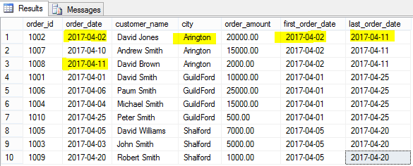
From the above image, we can clearly see that first order received on 2017-04-02 and last order received on 2017-04-11 for Arlington city and it works the same for other cities.
Useful Links
- Backup Types & Strategies for SQL Databases
- TechNet Article on the OVER Clause
- MSDN Article On DENSE_RANK
Other great articles from Ben
| How SQL Server selects a deadlock victim |
| How To Use Window Functions |

View all posts by Ben Richardson
- Working with the SQL MIN function in SQL Server - May 12, 2022
- SQL percentage calculation examples in SQL Server - January 19, 2022
- Working with Power BI report themes - February 25, 2021