
Introduction
A few months back I had been working on an interesting proof of concept for a human resources client (Mary Smith) who is the HR manager in a major hardware chain. The firm has a “ServiceNow” installation, with tables that stores employee ”hours worked”.
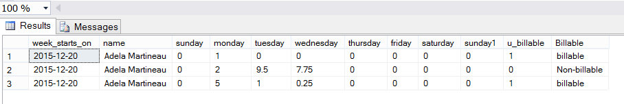
These hours are stored within the “Time Card” table and each employee has two rows within the table for each week. One row is for billable activities and the other for non-billable activities (such as travel and vacation time and getting to the customer site)
Weeks begin on Sunday and end on Saturday. Oft times these weekly records run cross month ends which as the reader can understand prove to be a big challenge when it comes to creating corporate reports.
A sample of this ‘cacophony’ may be seen below:
In today’s “fireside chat” we shall be developing the necessary queries and reports that will permit Mary to extract the necessary data on a fiscal month to month basis in order to provide senior management with the vital profit and loss information.
Thus, let’s get started.
Getting started
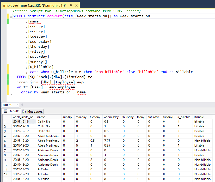
Opening SQL Server Management Studio, we open the SQLShack database. The query below provides the necessary raw data which is sourced from the “Employee” and “TimeCard” tables. We shall be working with this data.
Opening a new query we declare a few variables (see below).
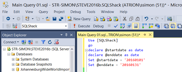
We declare a start and an end date variable (as may be seen above) and set the start of the period and the end of the period. Once complete and implemented, the start and end dates will be passed from the front end report to the stored procedure which we shall create from the code that we are developing.
As our point of departure, we create a small query that will decide which records we are looking for based on the user-defined start and end dates.
We remember that the start and end dates will be any day within a given weekly record. Dates that are colored green are the dates that we require (see below). Thus for the period 1/1/2016 through 1/31/2016 we require the “start” records shown below:
| WeekStartsON | Sunday | Monday | Tuesday | Wednesday | Thursday | Friday | Saturday |
| 12/27/2015 | 12/27/2015 | 12/28/2015 | 12/29/2015 | 12/30/2015 | 12/31/2015 | 1/1/2016 | 1/2/2016 |
PLUS all records up until and including the end record, shown below.
| WeekStartsON | Sunday | Monday | Tuesday | Wednesday | Thursday | Friday | Saturday |
| 1/31/2016 | 1/31/2016 | 2/1/2016 | 2/2/2016 | 2/3/2016 | 2/4/2016 | 2/5/2016 | 2/6/2016 |
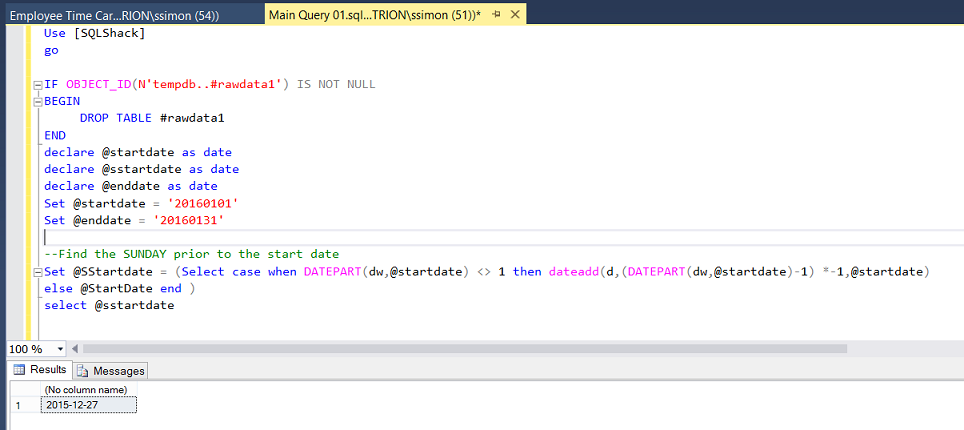
Our first task is to find the date of the SUNDAY immediately before our start date. As discussed immediately above, all records within the time card table start on a Sunday. In this case, as we are looking at 1/1/2016 as a start date and because 1/1/2016 is NOT a Sunday, we go back in time to ascertain the date of the Sunday, immediately before 1/1/2016 which turns out to be 12/27/2015 as may be seen in the screenshot below. The code to perform the necessary calculation may also be found below the screen shot.
|
1 2 3 4 |
Set @SStartdate = (Select case when DATEPART(dw,@startdate) <> 1 then dateadd(d,(DATEPART(dw,@startdate)-1) *-1,@startdate) else @StartDate end ) |
Our next task is to calculate the Saturday immediately after the end date. The end date is 1/31/2016. This date is a Sunday and to be all inclusive we must find the Saturday immediately after this date. This being 2/6/2016 as may be seen in the screen dump below. The code to ascertain this is also below the screenshot.

|
1 2 3 4 5 |
Set @EEnddate = (Select case when DATEPART(dw,@enddate) <> 7 then dateadd(d,(DATEPART(dw,@enddate)-1)*-1 ,@enddate) else dateadd(d,-6,@endDate) end ) Select @EEnddate |
Thus the first time card for each employee will be, for the week of December 27th 2015 and the last time card being for the week of January 31st 2016 (ending Saturday Feb 6th).
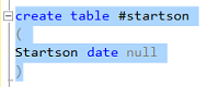
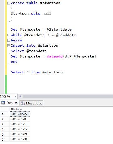
We now create a temporary table called #startson which will contain unique values of the suite of “Week_starts_on” that we are required to process (see above).
Populating our #startson table
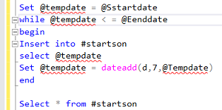
Utilizing a “while” loop, we insert the first date (our Sunday on or prior to the start date) into our #startson table. We then add 7 days to this date and the cycle begins again. The”trip –out” being when the incremented date is greater than the actual end date (provided by the client via the report).
Running this code snippet we find that we must consider records with the following Sunday’s as “week_starts_on” values:
Having obtained both the start of period and end of period dates, we are now in a position to pull the actual time card data including the “Week_starts_on” column and place these records into another temporary table.
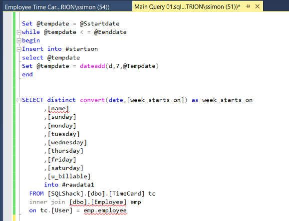
Now that we have the necessary data within our temporary table(s), we are in a position to manipulate the data and assemble it in a convenient fashion, utilizing a pivot table. The first and most important task is to rotate the data from this format
| WeekStartsOn | Sunday | Monday | Tuesday | Wednesday | Thursday | Friday | Saturday |
| 12/27/2015 | 2 hours | 3 | 1 | 8 | 9 | 4 | 2 |
To this format
| Week Starts On | Day of week | Hours Entered | DayEnteredNumber |
| 12/27/2015 | Sunday | 2 | 1 |
| 12/27/2015 | Monday | 3 | 2 |
| 12/27/2015 | Tuesday | 1 | 3 |
| 12/27/2015 | Wednesday | 8 | 4 |
| 12/27/2015 | Thursday | 9 | 5 |
| 12/27/2015 | Friday | 4 | 6 |
| 12/27/2015 | Saturday | 2 | 7 |
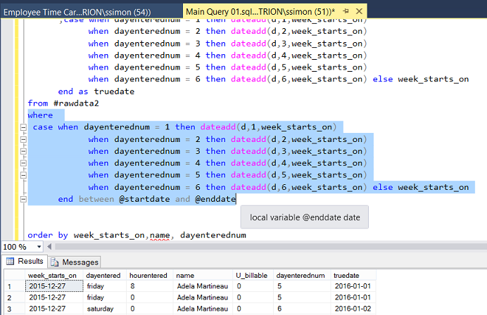
The code to achieve this may be seen in the screenshot below PLUS the code sample itself may be found in Addenda 1.

The astute reader will note the inner join of the main body of the code to the #startson temporary table that we created and populated above. This is an important fact, as the join (as discussed above) acts as a query predicate to ensure that we are pulling only those weekly time card relative to the period under consideration.
Our next task is to obtain the actual date upon which the hours were booked. Through the usage of the field “week_starts_on” and the field “dayenterednum”, we are able to calculate the proper calendar date.
In order to achieve this, we add one small piece of code to our query. This code utilizes the SQL Server date function “dateadd” (see below).
|
1 2 3 4 5 6 7 8 9 |
,case when dayenterednum = 1 then dateadd(d,1,week_starts_on) when dayenterednum = 2 then dateadd(d,2,week_starts_on) when dayenterednum = 3 then dateadd(d,3,week_starts_on) when dayenterednum = 4 then dateadd(d,4,week_starts_on) when dayenterednum = 5 then dateadd(d,5,week_starts_on) when dayenterednum = 6 then dateadd(d,6,week_starts_on) else week_starts_on end as truedate |
Running our query again, (after having included this piece of code) we note the new field called “truedate”(see below). This field contains the actual calendar date for this field.
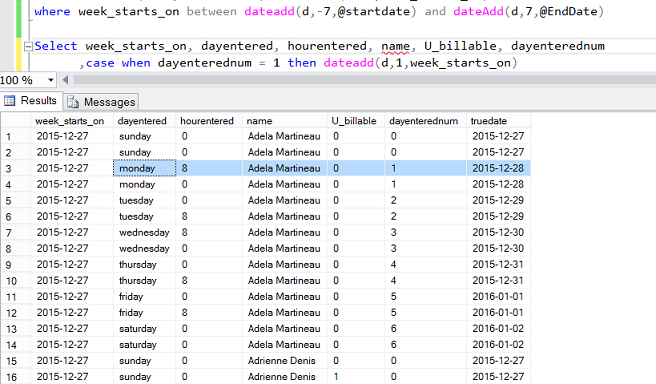
Now that we have our actual date field, all that remains to be done is to set the extraction predicate to pull “truedates” between the start and end date (see below).
Now that our coding is complete, our very last task is to create a stored procedure from our code. From the reports (that we are going to create), the user will pass a start and end date to our stored procedure.
Reporting
In order to create our report, we open either Visual Studio 2015 or SQL Server Data Tools 2010 or greater. Should you have never worked with Reporting Services or should you not feel comfortable creating a Reporting Services project, then please do have a look at one of our earlier chats where the “creation” process is described in detail.
Beer and the tabular model DO go together
We begin by creating a new Reporting Services project. We shall call our project “TimeCard”.
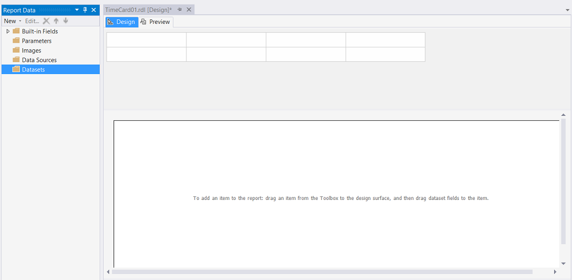
Our design surface is brought into view (see below).
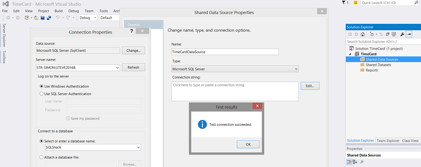
As we have done in our past “get togethers”, we create a shared data source which we call “TimeCardDataSource” (see below).
Having created our new shared data source, our next task is to create a new report.
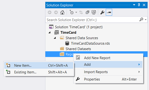
We right click on the “Report” tab and select “Add” and “New Item” (see below).
We are brought to the “Add New Item” menu. We select “Report” and give our report a name (see below).
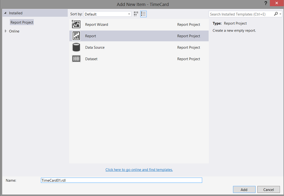
We click “Add” and we are returned to the drawing surface of our new report.
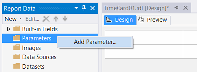
Our next task is to create a start date and an end date parameter.
Creating the necessary parameters
In order for our query to function correctly, we are required to pass a valid start and end date to the stored procedure. As discussed above we shall now create two parameters to do just this. We right-click on the Parameters tab and select “Add Parameter” (see below).
The “Report Parameter Properties” dialogue box is brought up (see below).
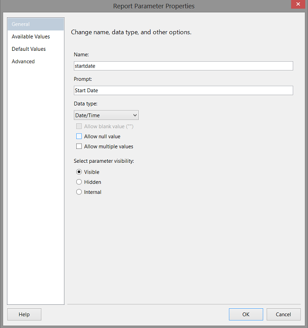
We name our parameter “startdate” and set the data type to date / time (see above).
We click “OK” to create the parameter.
We repeat the same process to create our “enddate” parameter. Our working surface and parameter frame should appear as follows.
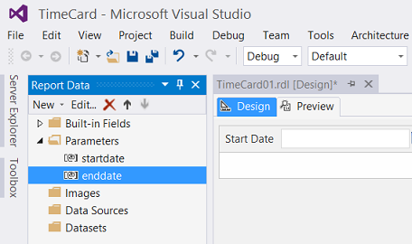
Finally, we require two local datasets. Before we do this, we are reminded that Mary would like to see two matrices on the report surface. One showing billable hours and the other non-billable hours, hence the need for two local datasets.
Creating our LOCAL datasets
As we shall have two matrices for Mary’s report, one showing billable hours and the other the non-billable hours, we are forced to apply different filters to each matrix. The astute reader will remember seeing a field called “u_billable”. This field is a boolean, 0 being non-billable and 1 being billable.
Creating the billable local dataset
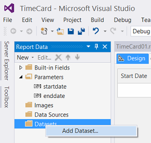
We right click upon the “Dataset” folder and select “Add (local) dataset” as shown above.
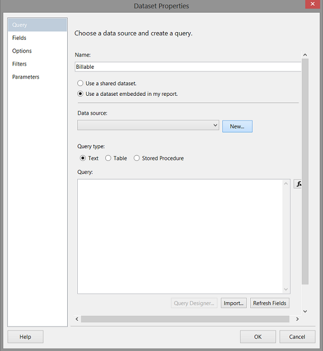
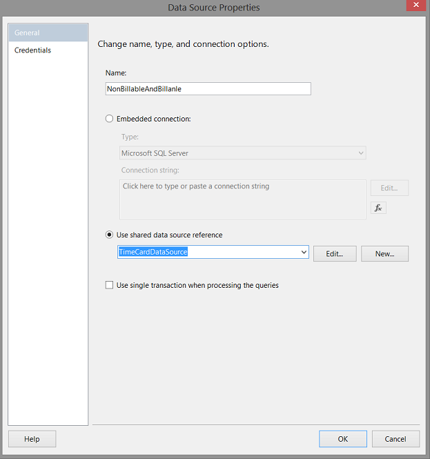
We opt to “Use a dataset embedded in my report” and click on the new button to create a new local data source which will utilize the shared data source which we created above.
Clicking “New”, the “Data Source Properties” dialog box opens. We opt to utilize the “Shared data source reference” as shown below. We click OK to exit this dialogue box.
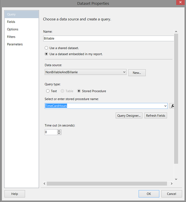
We are returned to our report surface with the “Dataset Properties” dialogue box showing. We select “Stored Procedure “ for the query type, choose our stored procedure, and then click the “Refresh Fields” button (see below).
We now click the “Fields” tab (see below).
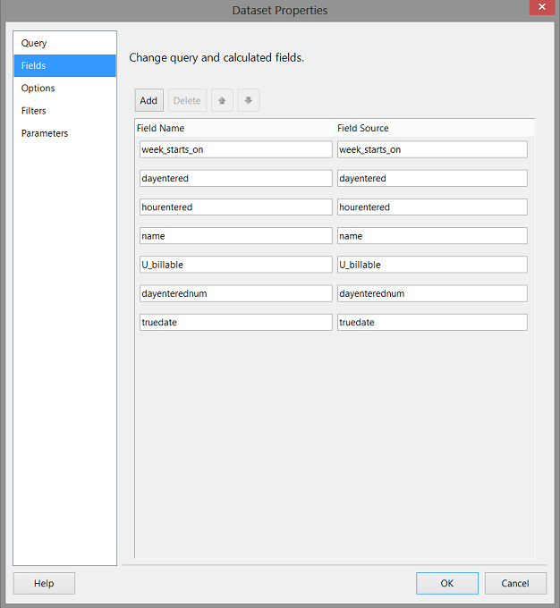
Clicking on the “Fields” tab we see the fields from the shared data source which in turn had obtained its field list from the stored procedure that we created (see above).
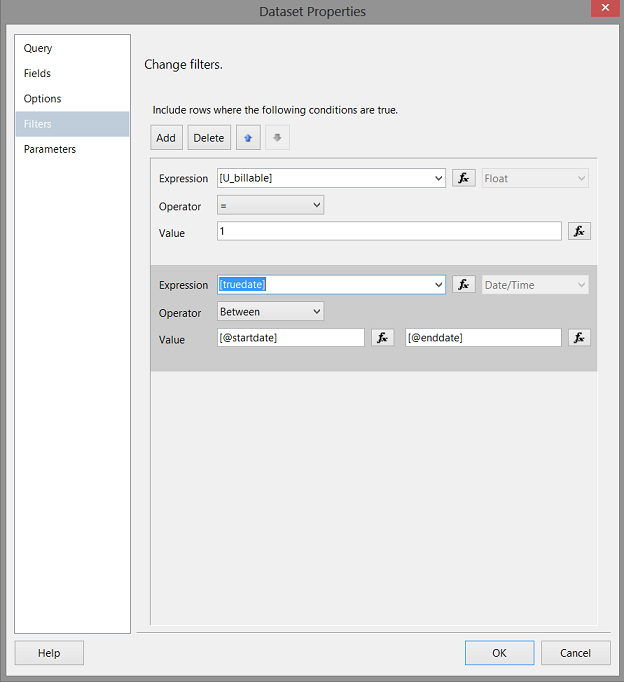
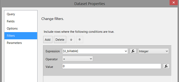
As this dataset will contain billable records, we must set a filter in order for our dataset to contain only those records that are billable(see above). We set the filter to look at the field “u_billable” and only extract those records whose “u_billable” value is 1. Further, we wish to extract only the records where the actual billing date is between the start and end dates.(see above). While this may seem a bit redundant, it ensures that the dataset displayed is exactly what the end user desires.
We click upon the “Parameters” tab to bring up the parameters dialogue box.
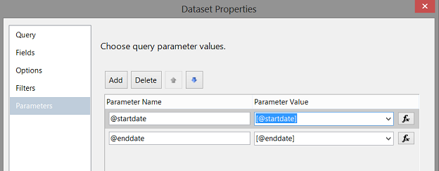
We ensure that the “Parameter Value” boxes are correctly populated (as may be seen above).
In a similar fashion, we are able to create the “nonbillable” local dataset. We note that “u_billable” is 0 in this case (see below).
Creating and populating our matrices
Now that our datasets have been created, we are in a position to view our results.
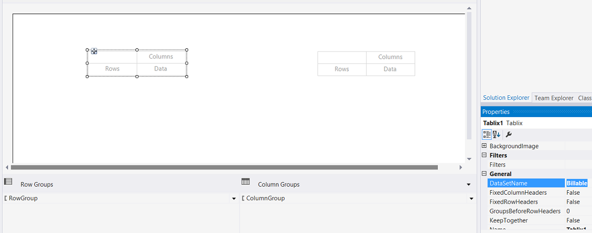
We drag two matrices from the toolbox and place them on the drawing surface (see below).
We click on the left-hand matrix and set the dataset property to point to the “billable” data set (see below).
Our next task is to define the “Row Group” aggregation. This will permit the totaling of the hours (per person) for each day.
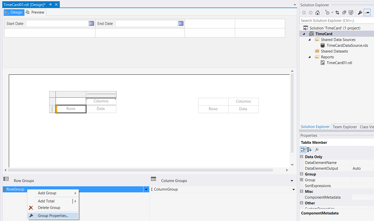
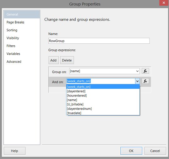
We right click on the “RowGroup” and select “Group Properties” (see above). The “Group Properties” dialogue box appears. We set the grouping on the employee name and the week (see below). It should be noted that we could just as well utilized the “Truedate” field.
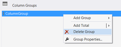
Processing the column grouping
We now right click upon the Column grouping and select “Delete Group” (see below).
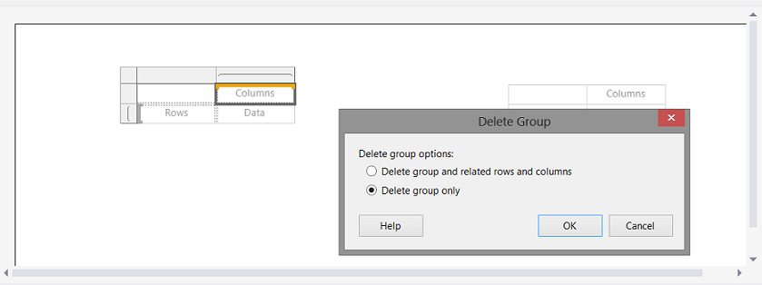
We are asked if we wish to delete the group and the related rows and columns OR merely to delete the groups. We opt to delete the groups only (see below).
Now that our matrix aggregation has been set, we are in a position to populate our “billable” matrix.
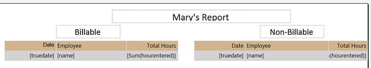
Our populated “Billable” matrix may be seen above. The astute reader will note that we utilized the field “truedate” as our date field. “truedate” is the actual date on which our hours were worked.
In a similar fashion, we repeat the same process for our “Non-Billable” hours, however, this time utilizing the non-billable dataset. The “non-billable” matrix is shown above as well.
Lastly, we apply a little make-up to the report by adding the main header and a sub-header for each of the matrices. We also apply some fill to our data boxes (see above).
Let us give our report a whirl
In order to prove to Mary that we have in fact created the report according to the correct specifications, we set the start date to 1/1/2016 and the end date to 1/31/ 2016. We click on the “Preview” tab and our report comes up (see below).

The end of period records may be seen below:
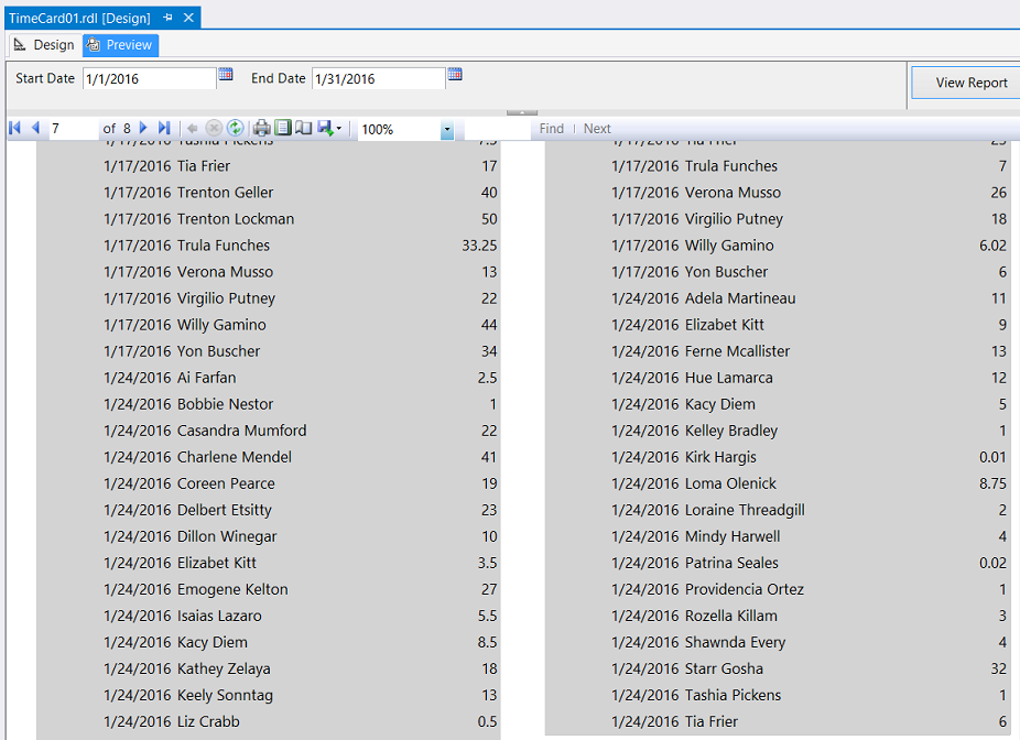
The reader will note that the extract begins on 1/1/2016 and ends on or before 1/31/2016.
Conclusions
So, we arrive at the end of another “fireside” chat. Oft times the format of the data (available for us to utilize) is not all that conducive to reporting. Mary’s SeviceNow installation’s “TimeCard” table has the daily chargeable and non-chargeable hours as seven columns within the table, a separate column for each day of the week. Each week begins on Sunday and the weekly records often will cross month ends. This makes it challenging to report on the results for a particular fiscal month. Pivot tables and date calculations help us make some sense out of this mess. They also help when it comes to report aggregation and ensuring that the decision maker is able to make efficient and effective decisions.
Happy programming and all the best!
Addenda 1
Pivot code
|
1 2 3 4 5 6 7 8 9 10 11 12 13 14 15 16 17 18 |
Select week_starts_on,dayentered, hourentered,name,u_billable, case when dayentered = 'monday' then 1 when dayentered = 'tuesday' then 2 when dayentered = 'wednesday' then 3 when dayentered = 'thursday' then 4 when dayentered = 'friday' then 5 when dayentered = 'saturday' then 6 when dayentered = 'sunday' then 0 end as dayenterednum into #rawdata2 from #rawdata1 unpivot ( hourentered for dayentered in (monday, tuesday, wednesday, thursday, friday, saturday, sunday) ) as unpvt inner join #startson ss on convert(date,ss.Startson) = convert(date,week_starts_on) where week_starts_on between dateadd(d,-7,@startdate) and dateAdd(d,7,@EndDate) Select * from #rawdata2 order by week_starts_on,name, dayenterednum |
References:
- Using PIVOT and UNPIVOT
- Create a Matrix (Report Builder and SSRS)
- Date and Time Data Types and Functions (Transact-SQL)
Steve has presented papers at 8 PASS Summits and one at PASS Europe 2009 and 2010. He has recently presented a Master Data Services presentation at the PASS Amsterdam Rally.
Steve has presented 5 papers at the Information Builders' Summits. He is a PASS regional mentor.
View all posts by Steve Simon
- Reporting in SQL Server – Using calculated Expressions within reports - December 19, 2016
- How to use Expressions within SQL Server Reporting Services to create efficient reports - December 9, 2016
- How to use SQL Server Data Quality Services to ensure the correct aggregation of data - November 9, 2016