
Description
Once collected, job performance metrics can be used for a variety of reporting needs, from locating jobs that are not performing well to finding optimal release windows, scheduling maintenance, or trending over time. These techniques allow us to maintain insight into parts of SQL Server that are often not monitored enough and prevent job-related emergencies before they become emergencies.
Introduction
Collecting job performance metrics provides us with the opportunity to then report on that data. In that realm, our imaginations are the only limiting factor.
We can create further fact tables to store aggregated metrics, perform gaps/islands analysis in order to find optimal job times or busy times, and ready data for consumption by reporting tools, such as SSRS or Power BI.
Using these tools & metrics, we can look at past data, in order to observe trends and forecast future job runtimes, allowing us to solve a performance problem before it becomes serious. We can use this data to alert on rogue jobs, or those that are performing well out of their typical boundaries. Data can be compared between servers or environments to hunt for differences that may indicate other unrelated processes that are not running optimally, or compare different hardware configurations on job performance.
The list of applications can continue for quite a while, and will vary depending on how you use SQL Server Agent, and the volume of jobs you create.
SQL Server Agent Job
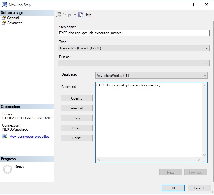
Previously, we have completed a script that can populate our metrics tables and clean them up as needed. We’ll encapsulate this TSQL into a stored procedure: dbo.usp_get_job_execution_metrics. This stored procedure, as well as all table & index creation scripts, can be downloaded at the end of this article.
To run this regularly, I’ll place the stored procedure execution into its own SQL Server Agent job, with a single step. Deletion of old data can be moved into an independent step if desired, but to keep things simple, I’ve opted to keep it in the main stored procedure. The job looks like this:
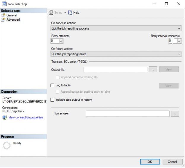
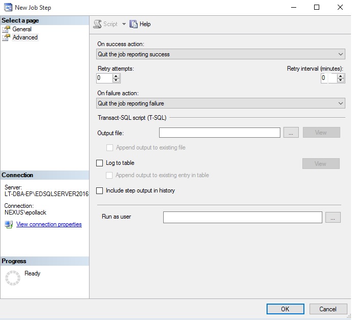
The advanced tab indicates that the job will complete and report success after the one (and only) step completes:
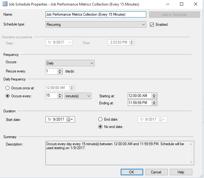
The schedule for this job is set to run it every 15 minutes. Feel free to adjust as needed based on the frequency of job executions and metrics needs on your system:
At this point, we have job collection tables, a collection stored procedure, and a job that can run regularly to collect and update our data. The last step is to consider how we will report on this data, and build the appropriate solution to present this data to us in a meaningful fashion!
Reporting on Job Performance Metrics
We’re now collecting job metrics, which can be very useful for monitoring and validating job history, but we can do much more with this data. To illustrate this, we will walk through a variety of metrics, showing how they can be calculated and returned to a user, report, or dashboard. The final version of this is included in a stored procedure that is attached to this article.
Now that we are ready to go, let’s consider a handful of metrics to report on:
-
Minimum, maximum, and average job runtime per day.
- Allows us to trend job performance over time in order to find patterns that require attention.
-
Complete job schedule details for a SQL Server.
- Useful for scheduling new jobs based on existing schedules.
-
Windows when jobs are not running, or when few are running.
- Helps in planning downtime and understand when quiet times are.
-
Alert on long/short running jobs when they become problematic.
- Catch problems before they become critical.
Job Runtime Averages
To facilitate the collection of this data, we can create a new table to store these aggregated metrics:
|
1 2 3 4 5 6 7 8 9 10 11 12 13 14 15 |
CREATE TABLE dbo.fact_daily_job_runtime_metrics ( fact_daily_job_runtime_metrics_ID INT NOT NULL IDENTITY(1,1) CONSTRAINT PK_fact_daily_job_runtime_metrics PRIMARY KEY CLUSTERED, Sql_Agent_Job_Id UNIQUEIDENTIFIER NOT NULL, Job_Run_Date DATE NOT NULL, Job_Run_Count INT NOT NULL, Job_Run_Failure_Count INT NOT NULL, Job_Run_Time_Minimum INT NULL, Job_Run_Time_Maximum INT NULL, Job_Run_Time_Average INT NULL ); CREATE NONCLUSTERED INDEX IX_fact_daily_job_runtime_metrics_Sql_Agent_Job_Id ON dbo.fact_daily_job_runtime_metrics (Sql_Agent_Job_Id); CREATE NONCLUSTERED INDEX IX_fact_daily_job_runtime_metrics_Job_Run_Date ON dbo.fact_daily_job_runtime_metrics (Job_Run_Date); |
With this table created, we can add some TSQL to our stored procedure to populate it:
|
1 2 3 4 5 6 7 8 9 10 11 12 13 14 15 16 17 18 19 20 21 22 23 24 25 26 |
DECLARE @Last_Complete_Averages_Collection_Date DATE; SELECT @Last_Complete_Averages_Collection_Date = MAX(fact_daily_job_runtime_metrics.Job_Run_Date) FROM dbo.fact_daily_job_runtime_metrics; SELECT @Last_Complete_Averages_Collection_Date = ISNULL(@Last_Complete_Averages_Collection_Date, '1/1/1900'); DELETE fact_daily_job_runtime_metrics FROM dbo.fact_daily_job_runtime_metrics WHERE fact_daily_job_runtime_metrics.Job_Run_Date >= @Last_Complete_Averages_Collection_Date; INSERT INTO dbo.fact_daily_job_runtime_metrics (Sql_Agent_Job_Id, Job_Run_Date, Job_Run_Count, Job_Run_Failure_Count, Job_Run_Time_Minimum, Job_Run_Time_Maximum, Job_Run_Time_Average) SELECT fact_job_run_time.Sql_Agent_Job_Id, CAST(fact_job_run_time.Job_Start_Datetime AS DATE) AS Job_Run_Date, COUNT(*) AS Job_Run_Count, SUM(CASE WHEN fact_job_run_time.Job_Status = 'Failure' THEN 1 ELSE 0 END) AS Job_Run_Failure_Count, MIN(fact_job_run_time.Job_Duration_Seconds) AS Job_Run_Time_Minimum, MAX(fact_job_run_time.Job_Duration_Seconds) AS Job_Run_Time_Maximum, AVG(fact_job_run_time.Job_Duration_Seconds) AS Job_Run_Time_Average FROM dbo.fact_job_run_time WHERE fact_job_run_time.Job_Start_Datetime >= @Last_Complete_Averages_Collection_Date GROUP BY fact_job_run_time.Sql_Agent_Job_Id, CAST(fact_job_run_time.Job_Start_Datetime AS DATE); |
Note that we remove an extra day of data prior to population that is from the last populated date. This is done as a safeguard against incomplete data, as we will need to recalculate averages on any data that is still being updated at the time of the job run. For reporting convenience, the job_id can be replaced with the job name, if desired.
The result of this script on my local server is a pile of job data that tells me about job executions per day per job:
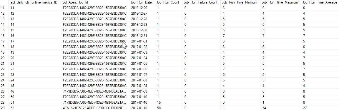
This data is aggregated by date, but could easily be updated to compute averages over a given hour, week, month, or other time period that is convenient. Similarly, we could create multiple fact tables to track metrics over multiple periods. Once data is aggregated, it may no longer be of use to you, in which case cleanup of older data can be performed more aggressively to improve performance and reduce disk usage.
Job Schedule Details
Returning a short list of all job/schedule relationships from our existing tables is almost trivial, now that the data is formatted in a friendly fashion:
|
1 2 3 4 5 6 7 8 9 10 11 12 13 14 15 16 17 18 19 20 |
SELECT dim_sql_agent_job.Sql_Agent_Job_Name, dim_sql_agent_schedule.Schedule_Name, dim_sql_agent_schedule.Schedule_Occurrence, dim_sql_agent_schedule.Schedule_Occurrence_Detail, dim_sql_agent_schedule.Schedule_Frequency, fact_sql_agent_schedule_assignment.Next_Run_Datetime FROM dbo.fact_sql_agent_schedule_assignment INNER JOIN dbo.dim_sql_agent_job ON fact_sql_agent_schedule_assignment.Sql_Agent_Job_Id = dim_sql_agent_job.Sql_Agent_Job_Id INNER JOIN dbo.dim_sql_agent_schedule ON fact_sql_agent_schedule_assignment.Schedule_Id = dim_sql_agent_schedule.Schedule_Id WHERE dim_sql_agent_job.Is_Enabled = 1 AND dim_sql_agent_job.Is_Deleted = 0 AND dim_sql_agent_schedule.Is_Enabled = 1 AND dim_sql_agent_schedule.Is_Deleted = 0 AND CURRENT_TIMESTAMP BETWEEN dim_sql_agent_schedule.Schedule_Start_Date AND dim_sql_agent_schedule.Schedule_End_Date ORDER BY fact_sql_agent_schedule_assignment.Next_Run_Datetime ASC; |
The result is a list of all job/schedule pairings, along with the next run time for the job:

We could also use a gaps/islands analysis on the job runtime data in order to determine the longest stretches of time when no jobs are running. Create a Dim_Time table, first, to store a joining table of minutes throughout the day:
|
1 2 3 4 5 6 7 8 9 10 11 12 13 14 15 16 17 18 19 20 21 22 |
CREATE TABLE dbo.Dim_Time ( Dim_Time TIME CONSTRAINT PK_Dim_Time PRIMARY KEY CLUSTERED); DECLARE @Current_Time TIME = '00:00'; INSERT INTO dbo.Dim_Time (Dim_Time) SELECT @Current_Time; SELECT @Current_Time = DATEADD(MINUTE, 1, @Current_Time); WHILE @Current_Time <= '23:59' AND @Current_Time > '00:00' BEGIN INSERT INTO dbo.Dim_Time (Dim_Time) SELECT @Current_Time; SELECT @Current_Time = DATEADD(MINUTE, 1, @Current_Time); END |
This data set could be changed to break down times on seconds, hours, or other time parts, if desired, including the addition of many days/dates/years. With this data, we can join duration data for a given day to it and get a picture of job activity over the course of a day:
|
1 2 3 4 5 6 7 8 9 10 11 12 |
DECLARE @Date_to_Check DATE = '1/10/2017'; DECLARE @Number_Of_Concurrent_Jobs INT = 0; SELECT Dim_Time FROM dbo.Dim_Time WHERE NOT EXISTS (SELECT * FROM dbo.fact_job_run_time WHERE Dim_Time.Dim_Time BETWEEN CAST(fact_job_run_time.Job_Start_Datetime AS TIME) AND CAST(fact_job_run_time.Job_End_Datetime AS TIME) AND CAST(fact_job_run_time.Job_Start_Datetime AS DATE) = @Date_to_Check) ORDER BY Dim_Time.Dim_Time; |
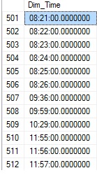
We can take this logic a bit further and analyze our set of times and report back on how many jobs run at any one time and filter accordingly. This would allow for a bit more intelligent scheduling where we could report on periods with nothing running, 1 job running, 2 jobs running, etc…Presumably, the more processes we tolerate running, the more windows of availability there will be for the scheduling of new jobs. To get a data set that shows each time (by second) and the number of concurrent jobs, we can run the following TSQL:
|
1 2 3 4 5 6 7 8 9 10 11 12 13 14 15 16 17 18 19 20 21 22 23 |
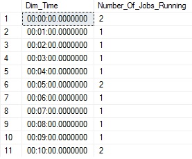
DECLARE @Date_to_Check DATE = '1/10/2017'; WITH CTE_JOB_DATA AS ( SELECT CAST(fact_job_run_time.Job_Start_Datetime AS TIME) AS Job_Start_time, CAST(fact_job_run_time.Job_End_Datetime AS TIME) AS Job_End_time FROM dbo.fact_job_run_time WHERE CAST(fact_job_run_time.Job_Start_Datetime AS DATE) = @Date_to_Check), CTE_DIM_TIME AS ( SELECT Dim_Time, COUNT(*) AS Number_Of_Jobs_Running FROM dbo.Dim_Time INNER JOIN CTE_JOB_DATA ON Dim_Time.Dim_Time BETWEEN CTE_JOB_DATA.Job_Start_time AND CTE_JOB_DATA.Job_End_time GROUP BY Dim_Time) SELECT * INTO #Job_Run_Data FROM CTE_DIM_TIME; SELECT * FROM #Job_Run_Data; |
This script will take all times in the dim_time table and compare them to our job performance data, returning a count for each minute of the jobs running at that time, only for those times in which jobs were running:
From here, we could constrain the results to allow for one job running (or 2, or 3) and perform an islands analysis on it in order to determine the optimal time to run a job. For this example, we’ll allow for a single running job. To facilitate a more efficient query, the results from above will be used, pulling from the temp table, rather than creating one monster query with both aggregation and islands analysis contained within:
|
1 2 3 4 5 6 7 8 9 10 11 12 13 14 15 16 17 18 19 20 21 22 23 24 25 26 27 28 29 30 31 32 33 34 35 36 37 38 39 40 41 42 43 44 |
WITH CTE_JOB_RUN_DATA AS ( SELECT Dim_Time.Dim_Time, ISNULL(Job_Run_Data.Number_Of_Jobs_Running, 0) AS Number_Of_Jobs_Running FROM Dim_Time LEFT JOIN #Job_Run_Data Job_Run_Data ON Dim_Time.Dim_Time = Job_Run_Data.Dim_Time ), ISLAND_START AS ( SELECT Job_Run_Data.Dim_Time, ROW_NUMBER() OVER(ORDER BY Job_Run_Data.Dim_Time ASC) AS Row_Num FROM CTE_JOB_RUN_DATA Job_Run_Data WHERE Job_Run_Data.Number_Of_Jobs_Running <= 1 AND EXISTS ( SELECT * FROM CTE_JOB_RUN_DATA Previous_Run WHERE Previous_Run.Dim_Time = DATEADD(MINUTE, -1, Job_Run_Data.Dim_Time) AND Previous_Run.Number_Of_Jobs_Running > 1) ), ISLAND_END AS ( SELECT Job_Run_Data.Dim_Time, ROW_NUMBER() OVER(ORDER BY Job_Run_Data.Dim_Time ASC) AS Row_Num FROM CTE_JOB_RUN_DATA Job_Run_Data WHERE Job_Run_Data.Number_Of_Jobs_Running <= 1 AND EXISTS ( SELECT * FROM CTE_JOB_RUN_DATA Next_Run WHERE Next_Run.Dim_Time = DATEADD(MINUTE, 1, Job_Run_Data.Dim_Time) AND Next_Run.Number_Of_Jobs_Running > 1) ) SELECT ISLAND_START.Dim_Time AS Job_Time_Island_Start, ISLAND_END.Dim_Time AS Job_Time_Island_End, (SELECT COUNT(*) FROM Dim_Time Island_Time_Minutes WHERE Island_Time_ Minutes.Dim_Time BETWEEN ISLAND_START.Dim_Time AND ISLAND_END.Dim_Time) AS Island_Time_Minutes FROM ISLAND_START INNER JOIN ISLAND_END ON ISLAND_START.Row_Num = ISLAND_END.Row_Num ORDER BY ISLAND_START.Dim_Time; |
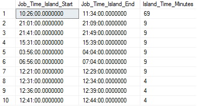
The result of this query is a set of acceptable times to potentially schedule a new job, the start and end times for each window, and the length of the window (In minutes). If we didn’t have a reliable dim_time table, or a uniform increment of minutes as we do here, an additional ROW_NUMBER could be added to CTE_JOB_RUN_DATA to normalize messy data and allow for easy analysis across it. The results look like this:
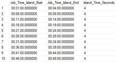
This isn’t the most useful view as we are getting lots of duplication. What we ideally want to see are the longest time windows first. To get this ordering, we can implement another CTE or put the above results into a second temp table, from where we can freely query the small result set. For this example, I’ve put the above data into a temp table called #Job_Runtime_Windows, and then run the query below:
|
1 2 3 4 5 6 |
SELECT * FROM #Job_Runtime_Windows ORDER BY Island_Time_Minutes DESC; |
The results show a specific time frame that appears ideal for the addition of a new job:
Long and Short Running Jobs
Another area of concern are jobs that run for an abnormal amount of time. To accurately alert or report on these, we need to have a fairly good idea of what is normal or not normal, both in terms of absolute and relative metrics comparisons.
For example, we could create a rule that states, “Any job that runs for 50% longer than its average time should be flagged as long-running”. If a job typically takes 500ms seconds to execute, and one day suddenly takes 1s, we likely won’t want an alert firing, as the difference is still very small. In other words, we would want to consider a threshold for runtime increases to ensure we don’t get false-alarms, such as only considering jobs that take 5 minutes or more to execute.
Earlier, we wrote a script that would populate fact_daily_job_runtime_metrics, which provides us with a table of daily run stats, which can be used as a baseline to compare against. Since that table includes average values and counts, we can compute averages over any time span (weeks, months, etc…). We then can look at all job runs for today, and report on any that are taking too long to run:
|
1 2 3 4 5 6 7 8 9 10 11 12 13 14 15 16 17 18 19 20 21 22 23 24 25 26 |
WITH CTE_AVERAGE_JOB_RUNTIME AS ( SELECT dim_sql_agent_job.Sql_Agent_Job_Name, dim_sql_agent_job.Sql_Agent_Job_Id, SUM(fact_daily_job_runtime_metrics.Job_Run_Count) AS Job_Run_Count, SUM(fact_daily_job_runtime_metrics.Job_Run_Time_Average * fact_daily_job_runtime_metrics.Job_Run_Count) / SUM(fact_daily_job_runtime_metrics.Job_Run_Count) AS Job_Run_Time_Average FROM dbo.fact_daily_job_runtime_metrics INNER JOIN dbo.dim_sql_agent_job ON fact_daily_job_runtime_metrics.Sql_Agent_Job_Id = dim_sql_agent_job.Sql_Agent_Job_Id GROUP BY dim_sql_agent_job.Sql_Agent_Job_Id, dim_sql_agent_job.Sql_Agent_Job_Name) SELECT CTE_AVERAGE_JOB_RUNTIME.Sql_Agent_Job_Name, fact_job_run_time.Job_Start_Datetime, fact_job_run_time.Job_End_Datetime, fact_job_run_time.Job_Duration_Seconds, fact_job_run_time.Job_Status, CTE_AVERAGE_JOB_RUNTIME.Job_Run_Count, CTE_AVERAGE_JOB_RUNTIME.Job_Run_Time_Average FROM dbo.fact_job_run_time INNER JOIN CTE_AVERAGE_JOB_RUNTIME ON CTE_AVERAGE_JOB_RUNTIME.Sql_Agent_Job_Id = fact_job_run_time.Sql_Agent_Job_Id WHERE fact_job_run_time.Job_Start_Datetime >= CAST(CURRENT_TIMESTAMP AS DATE) AND CTE_AVERAGE_JOB_RUNTIME.Job_Run_Time_Average > 15 AND fact_job_run_time.Job_Duration_Seconds > CTE_AVERAGE_JOB_RUNTIME.Job_Run_Time_Average * 2; |
This script computes an average all-time for our duration data. If desired, we could constrain it to the past week, month, quarter, or whatever other time frame seems appropriate for “recent” data. We then compare today’s job runtimes to the average and if any individual job took more than double the average, a row is returned. We intentionally ignore any jobs that average 15 seconds or less, since they would likely cause unnecessary noise. This filter can also be adjusted to be more or less aggressive, to omit specific types of jobs, or otherwise clean up results such that no false alerts are generated. The results on my local server look like this:
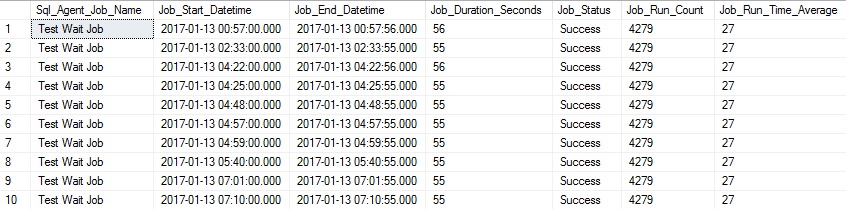
The results show each instance of a job that took longer than double the average run time (27 seconds in this case) and some pertinent details for it. This reporting can be sent out whenever needed, and could even be alerted on, if such a need arose. The metrics that determine a long running job are completely customizable. We can similarly filter for short running jobs—those that execute extremely quickly, and therefore may not be performing the usual amount of work. Adjusting this is as simple as changing the criteria of the WHERE clause above to:
- Run for a different time frame, multiple days, a fraction of a day, etc…
- Set a minimum or maximum threshold to check.
- Eliminate edge cases, such as jobs that are supposed to be very quick.
- Create more liberal boundaries for jobs that are known to be erratic. Statistics such as standard deviation can be useful in better gauging how inconsistent results are, in order to avoid hard-coding job details.
Performance
With queries that are full of aggregation, common table expressions, table scans, and tiered queries, it is only natural to inquire about performance.
In general, the processes that write this data are relatively speedy and will do what they need to quickly and without introducing any latency or resource drain on the system they are run. The reporting queries generally rely on table scans and have the potential to get slow. While not problematic, this is the primary reason that we separate our reporting data into new, customized tables and generate further reporting tables as we determine a need for more metrics. For example, we create dbo.fact_daily_job_runtime_metrics and store daily averages in this table, rather than run our aggregations directly against our more granular data, or against the MSDB system views.
This provides us with more control, and the ability to design and structure the metrics tables to meet our custom needs. Include only the columns we need, with supporting indexes, and reports that are helpful. Any extraneous data in MSDB can be left out, and we only need to maintain as much data as we wish. Oftentimes, the granular data we store in fact_job_run_time and fact_step_job_run_time can be aggregated into more compact tables, such as the daily runtime metrics table referenced above. Once this data is crunched for the day, we need only keep it for a short while and then delete it. For some use-cases, a week or two may be all that is necessary to keep. If all we care about are metrics and will never review the detail data, then a single day of retention may be sufficient.
By controlling the data size and maintaining only the most useful metrics and relevant data, we can ensure that our reports run quickly. Even the Job duration/islands analysis, comprised of 3 cascading CTEs, can be fast, so long as the underlying data is kept simple and streamlined. Consider moving data to temporary tables when crunching more complex metrics, instead repeatedly accessing a large fact table.
In no examples here was performance a significant concern, but knowing how to deal with large reporting tables effectively can help in keeping things moving along efficiently. We do not want to suffer the irony of a reporting job that monitors job performance and becomes the resource hog on our server 🙂
Customization
We can easily customize what metrics we collect, as shows previously, but our ability to tailor reports to our own SQL Server environments is even more significant. Data presented here is the tip of the iceberg. With the underlying data present, we could delve into many other areas, such as failed job details, runtime of job steps, automatic or semi-automatic job scheduling, and much more! The techniques to accomplish tasks such as these will be the same as presented here.
Be creative and always start with questions prior to building a reporting structure. Decide exactly what you are looking for and build the collection routines and reporting infrastructure to answer those questions. If anything I’ve presented is unnecessary, feel free to remove it.
Conclusion
The techniques above demonstrate some simple ways in which we can collect useful job performance metrics, such as calculating averages over the course of a day. They also show how we can apply more advanced TSQL towards scheduling insight, using an islands analysis over job runtime data in order to determine when the most or fewest jobs are running.
If you come up with any slick ways to use or report on this data, feel free to contact me and let me know! I love seeing the creative ways in which seemingly simple problems can be turned into elegant or brilliant solutions!

In his free time, Ed enjoys video games, sci-fi & fantasy, traveling, and being as big of a geek as his friends will tolerate.
View all posts by Ed Pollack
- SQL Server Database Metrics - October 2, 2019
- Using SQL Server Database Metrics to Predict Application Problems - September 27, 2019
- SQL Injection: Detection and prevention - August 30, 2019