Introduction

In our last get together I mentioned that oft times SQL Server reports are created due to a dire business need to be used once and never again. Further, some reports that we believe are not often used could be “top of the pops” unbeknown to us. A guess as to a number of times a report is used per month, in addition to the statistics behind each report should not be guesswork, but rather monitored actively to ensure that frequently used reports are both efficient and effective. Further, those reports that are either not used or have not been run in quite some time, should perhaps be removed in order to keep the server clean and not cluttered.

In today’s get together, we shall be constructing a quick and dirty SQL Server Reporting Services application that will track report usage and runtime statistics to ensure that your servers are offering your users the best of both worlds, i.e. effective reports, cleaner servers and faster access time.

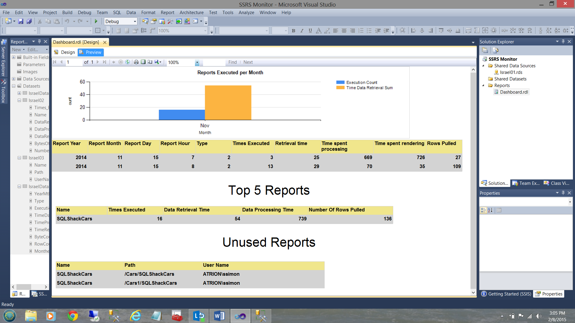
Our finished dashboard will look similar to the one shown below.

Let’s get started!!

Getting started

We start by opening Visual Studio and creating a new Reporting Services Project.

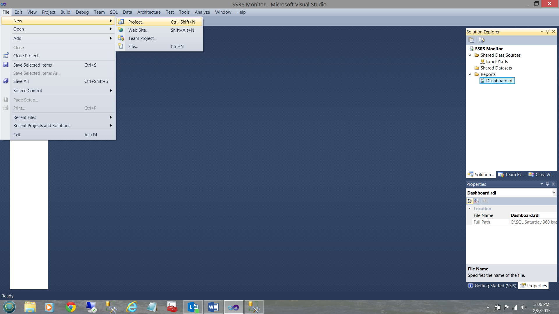
We select “New” then “Project” (see above).

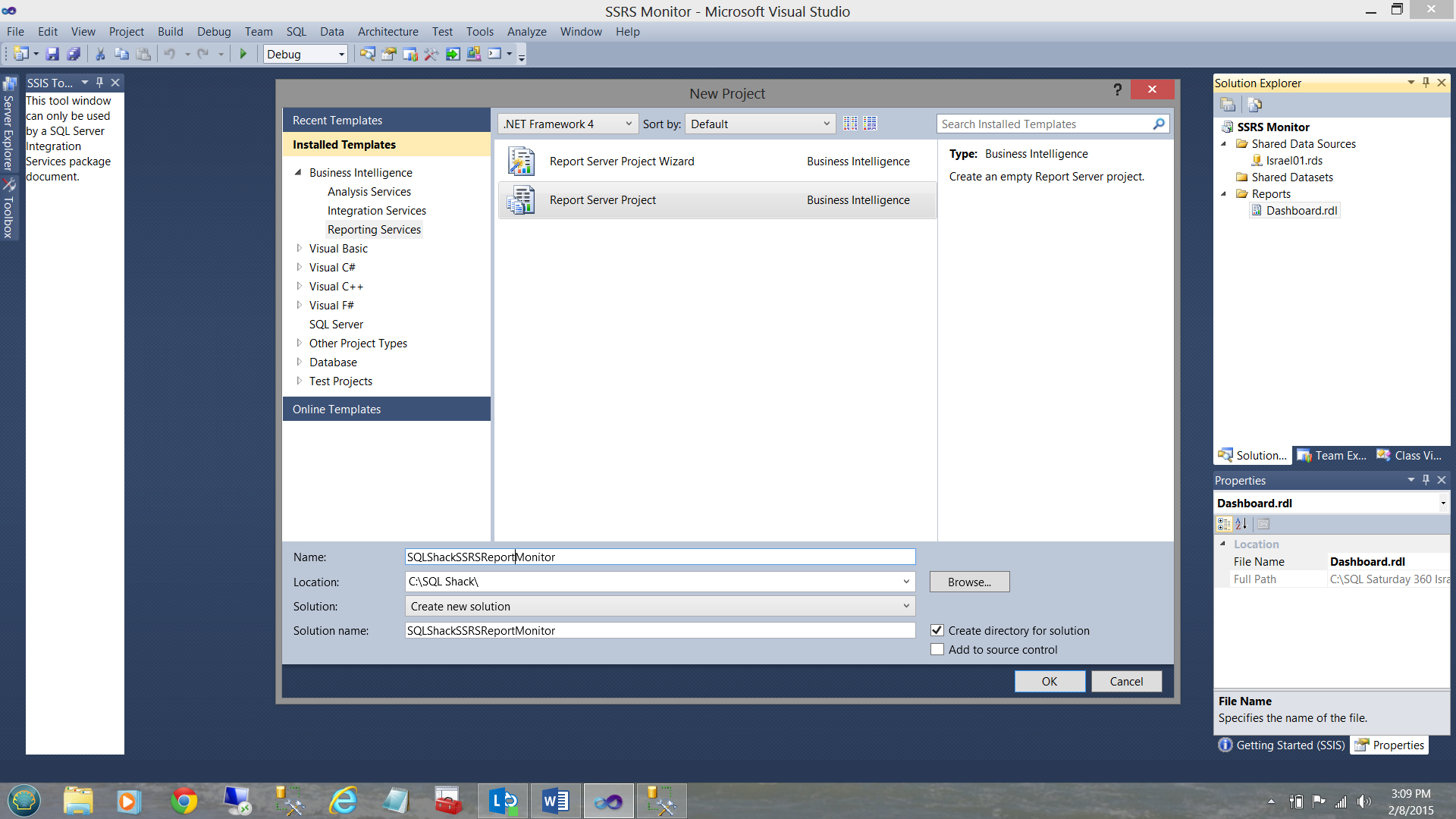
Next, we set the project type to Reporting Services and select a “Report Server Project” (see above). We click OK to continue.

We now find ourselves at our Reporting Services workspace.

Our first task is to create a new “Shared Data Source”. As we have discussed in many past articles, a “Data Source” may be likened to a water hose connecting the house water tap (the database) to the pot plants 20m from the house (the datasets behind our charts/matrices etc.).

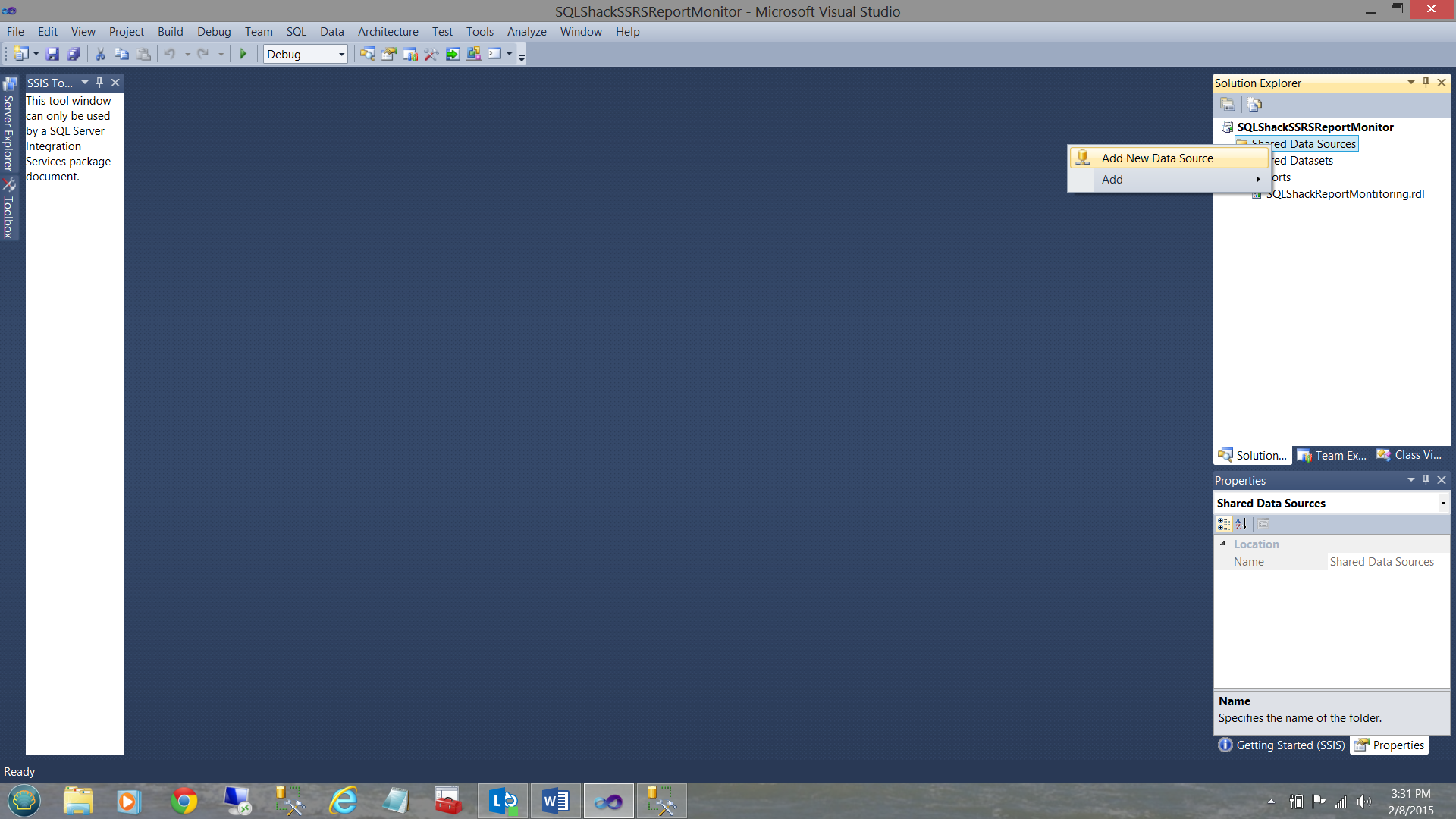
To begin we right-click on the “Shared Data Sources” folder and select “Add New Data Source”.

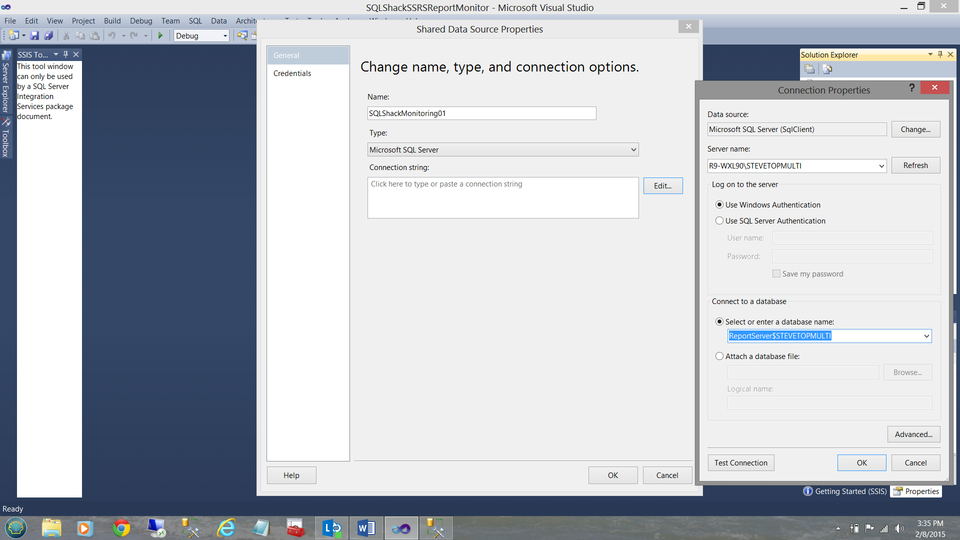
The “Shared Data Source” dialogue box is brought up. We give our data source a name “SQLShackMonitoring01”. Next, we click the “Edit” button to the right of the “Connection string” text box. The “Connection Properties” dialogue box is then opened and we configure our server name and NOTE that the database selected is our “ReportServer$STEVETOPMULTI” (see above and to the right).

Testing the connection, we see that all is in order (see above). We click OK, OK and OK again to exit the “Data source configuration” screens.

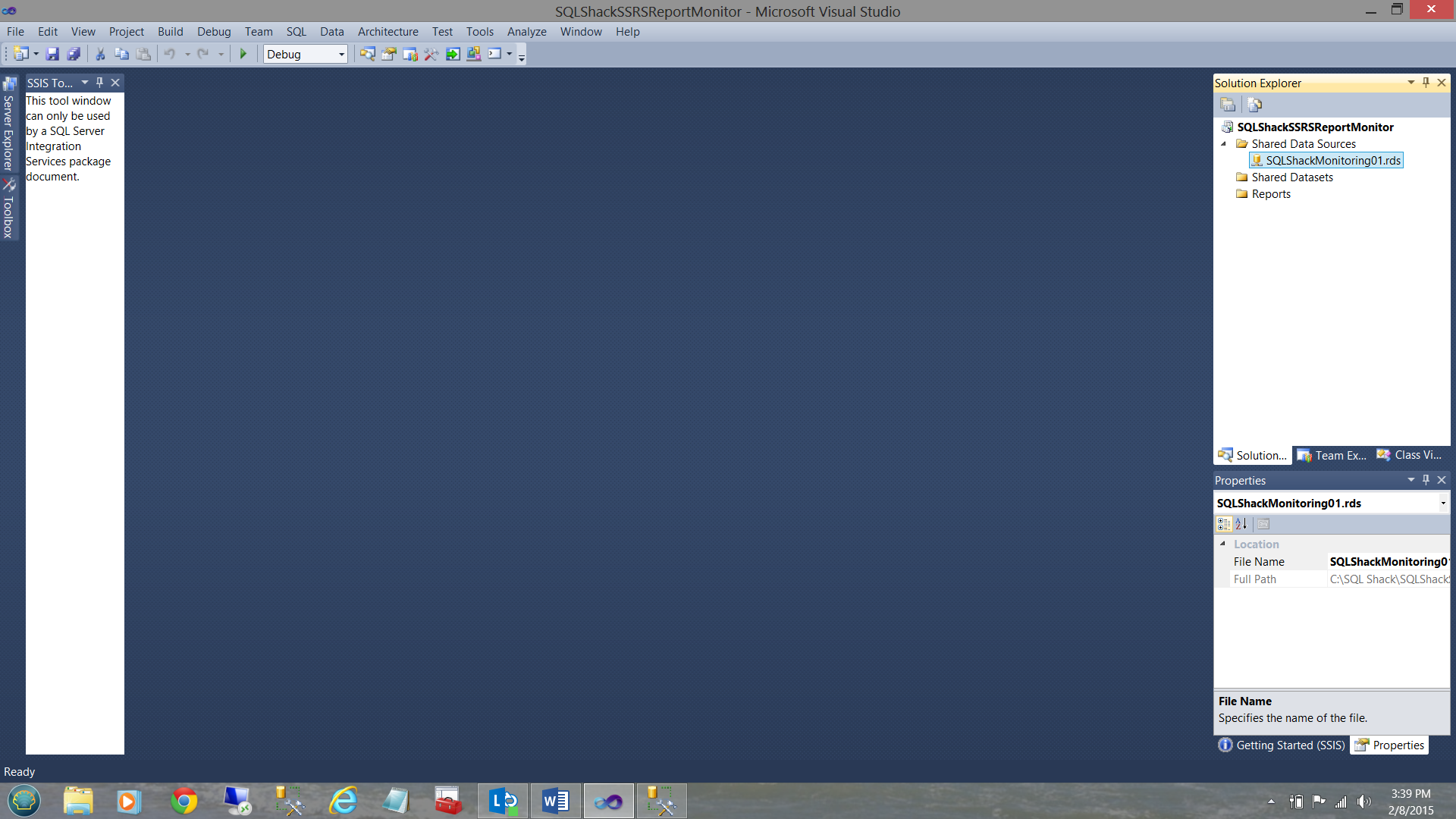
The reader will note that we have been returned to our work surface and the new data source is present in the top right of the screenshot above.

To find more detailed instructions on configuring data sources and creating datasets, the reader is referred to one of my previous articles entitled “Life is full of choices”

/life-full-choices/

Creating our “monitoring” report

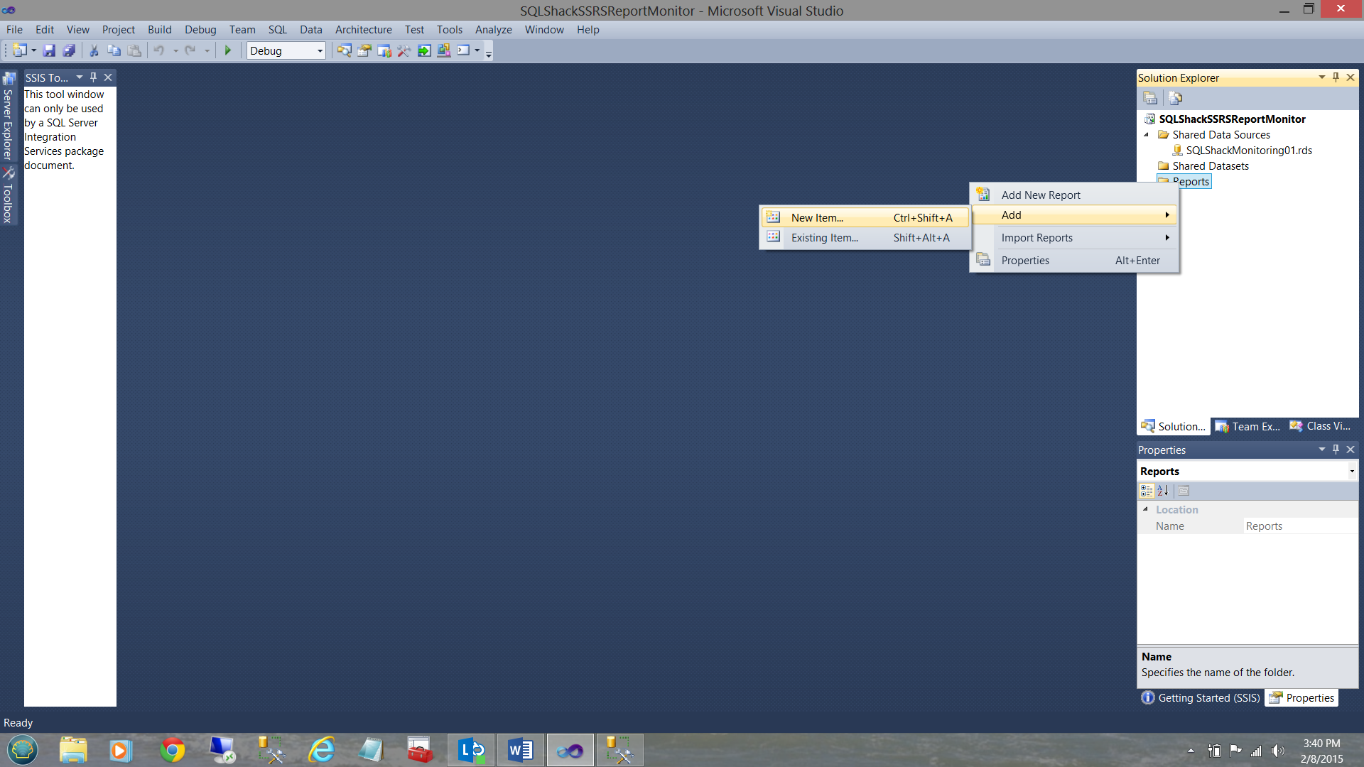
We start the development process by creating our one and only report. We right-click on the “Reports” directory (see above and to the right) and select “Add” and “New Item” from the context menu (see above).

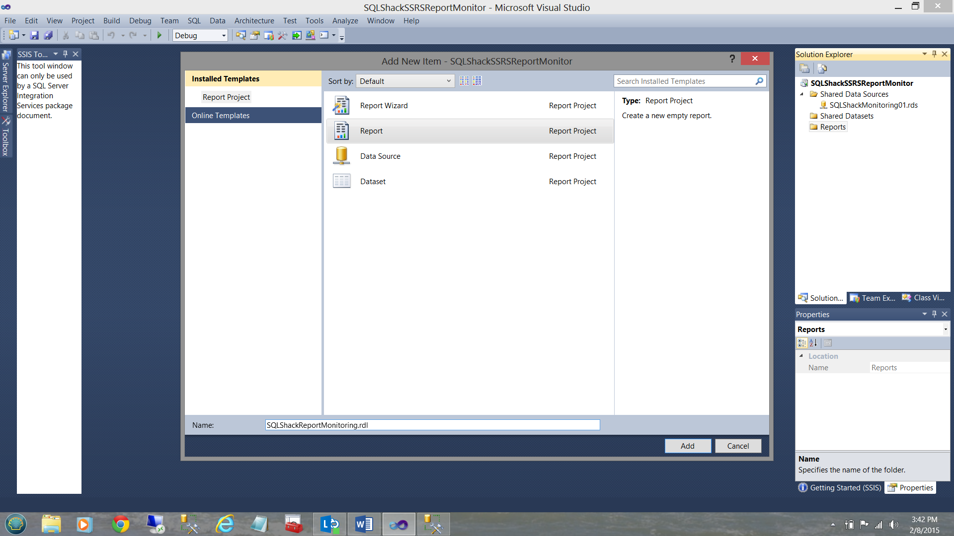
The “Add New Item” window is brought up. We select “Report” and give our report the name “SQLShackReportMonitoring’. We click “Add”.

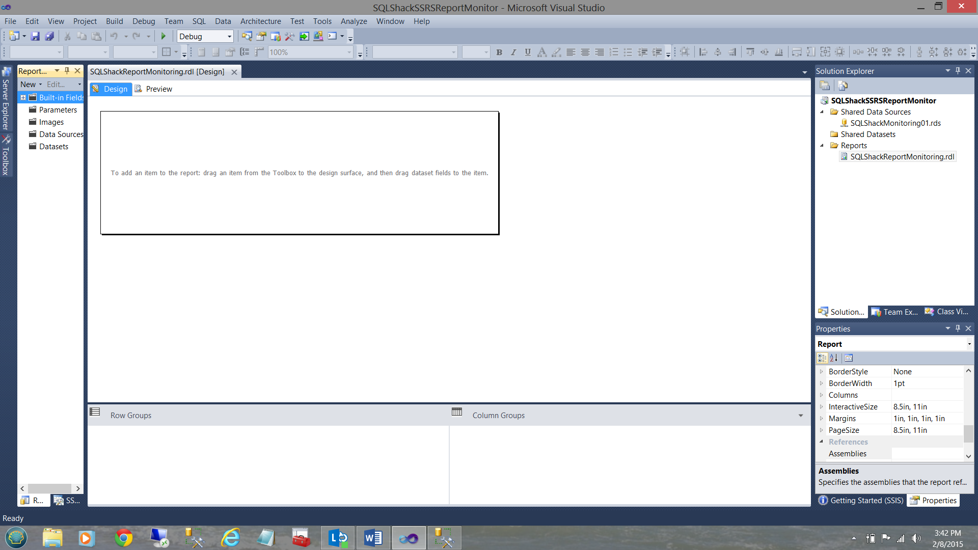
Our report drawing surface is brought into view (see above).

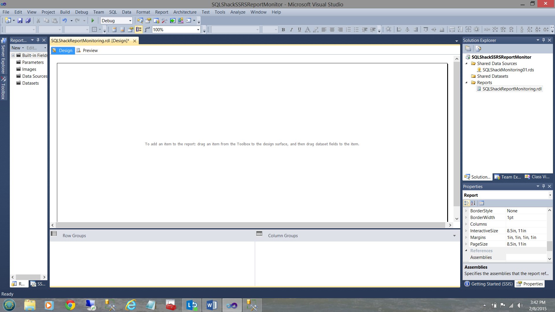
Having resized the drawing surface, we are ready to get started.

Creating the necessary stored procedures

As most of you know by now, my favorite approach to pulling report data from the database tables is via stored procedures as opposed to utilizing T-SQL commands. Stored procedures are definitely more optimal, clean and compact.

In the screen dump shown below, we note that we once again utilize a report that we created in a previous “get together”.

/life-full-choices/

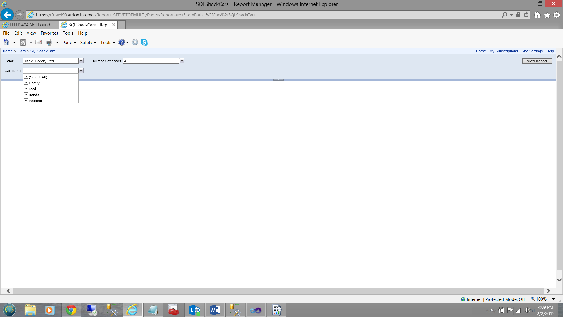
This report permits the user to find the models, colors, and a number of doors of automobiles available for sale at “SQLShackFinancial”. Running reports from the Report Server creates statistical data and it is this data that we shall be pulling for our monitoring report.

I have taken the liberty of running this report a few times to generate some data.

Stored Procedure 1 “Reports Executed per Month”

Running our “Reports Executed per Month” query, we find that a number of times that the “Cars” report was run three times in February 2015 (see below).

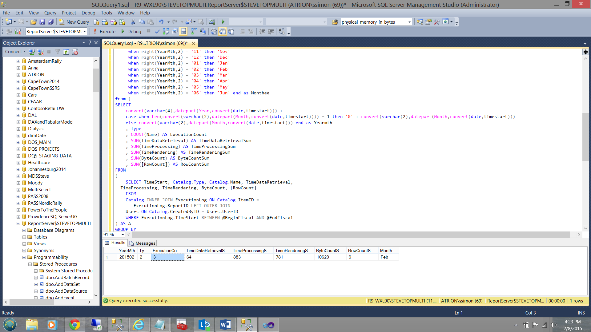
Further, the query gives us the “reporting period” year and month, the report execution count, the time spent processing the reports, the byte count of data passed back, the number of rows returned by the query and finally the month name of the reporting period. All of which are interesting and valuable statistics.

The code for this query may be found in Addenda 1.

Stored Procedure 2 “Statistics for Matrix”

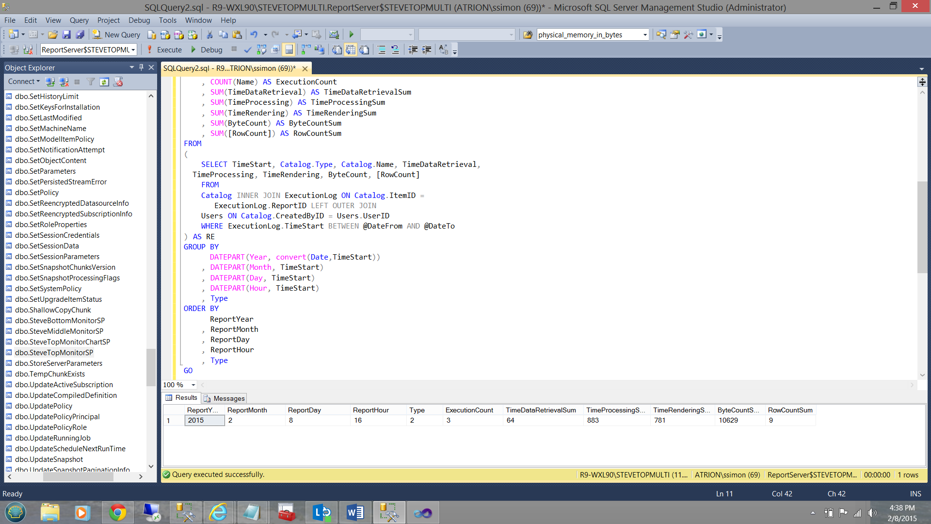
This query / stored procedure will pull the following statistics for each and every report run on our server for the current time period. The reader will note that the data returned includes the report year, the report month, the report day, the type of object that caused the counter to increment (2 is a report). The reader may follow up on this one with the following link.

https://social.msdn.microsoft.com/Forums/sqlserver/en-US/60dd3392-42d8-4dc4-b8e6-15e9aeaad29e/table-explaination-for-dbocatalog-table-in-reportserver-database

The execution count, the total time for the data retrieval and processing time are also returned along with the number of bytes transferred and the TOTAL number of rows that were returned.

The code for this procedure may be found in Addenda 2.

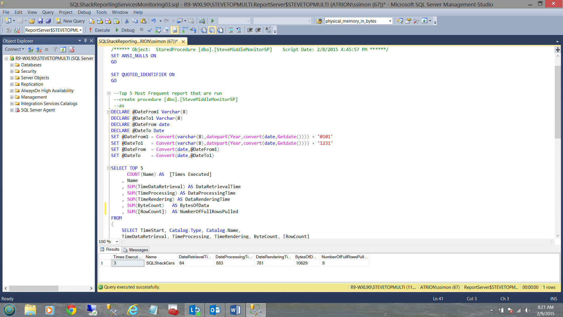
Stored Procedure 3 “Top 5 Reports”

Our next stored procedure will be utilized to obtain the five most popular reports. This is a great feature as it tells us which reports our users find most useful in their day to day activities.

The code listing may be found in Addenda 3.

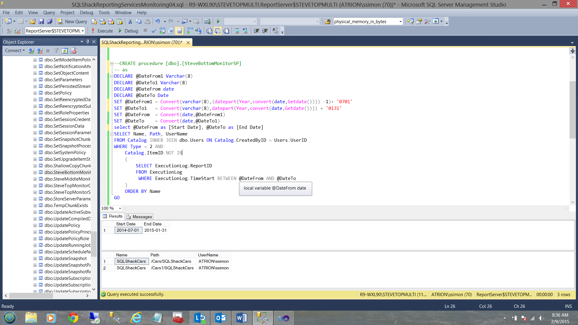
Stored Procedure 4 “Unused Reports”

This stored procedure is perhaps the most important to us. It will tell us which reports have not been run during the current period of time. This “period” could be the current month. The stored procedure gives us the name of the report, the path of the report and the ID of the users that last called the report.

The code listing for this stored procedure may be found in Addenda 4.

Meanwhile, back in our Reporting Server project

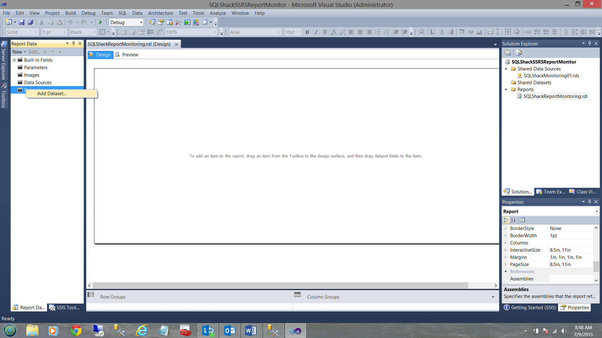
Having now constructed the four necessary stored procedures that are required to complete our monitoring project, we must now add the first of four local / embedded data set. We right-click on the Dataset folder and select “Add Dataset” (see above).

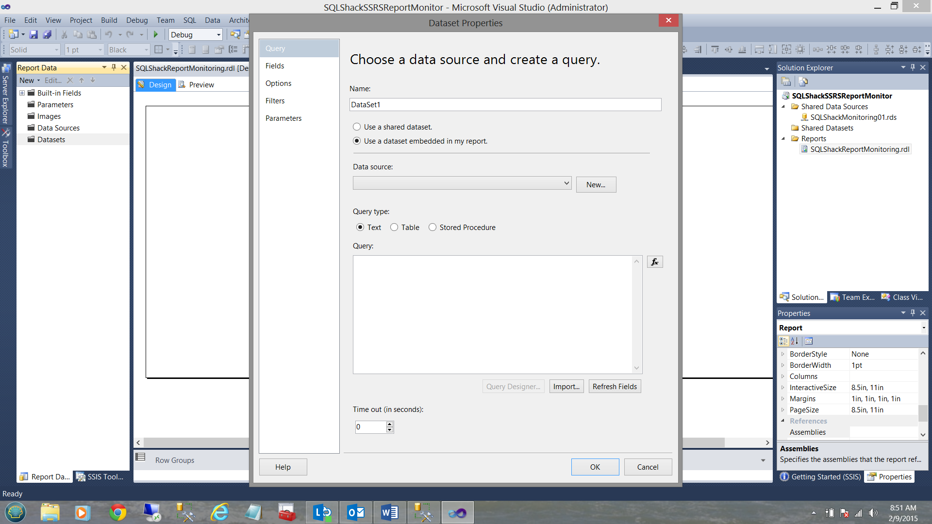
The Dataset Properties dialogue box opens. We select the “Use a dataset embedded in my report” option. We then click the “New” button to the right of the “Data Source” drop down box to create a new LOCAL data source (see above).

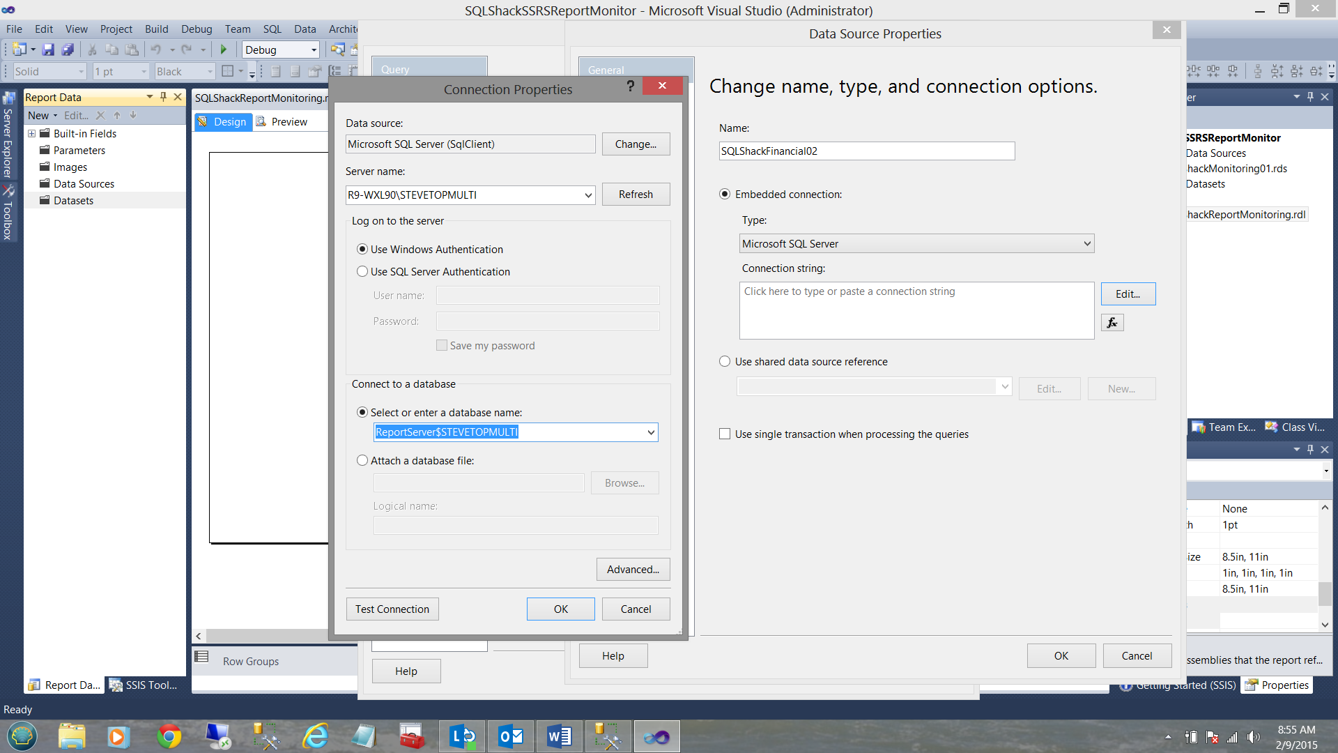
The “Change name, type, and connection options” dialogue box is brought into view. We give our connection a name “SQLShackFinancial02” and click the edit button to bring up the “Connection Properties” dialogue box where we enter our server name and “Select or enter a database name”. In our case, we select “ReportServer$STEVETOPMULTI” (see above). We click OK, OK and OK to exit the “Connection” dialogue pages.

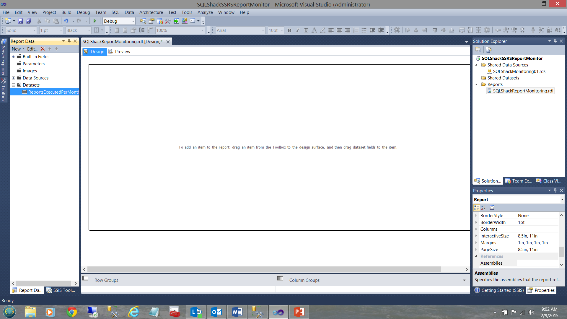
We find ourselves back at our drawing surface with our newly created dataset (see above). We must now configure this dataset.

Double clicking on the dataset, brings up the “Dataset Properties” dialogue box (once again).

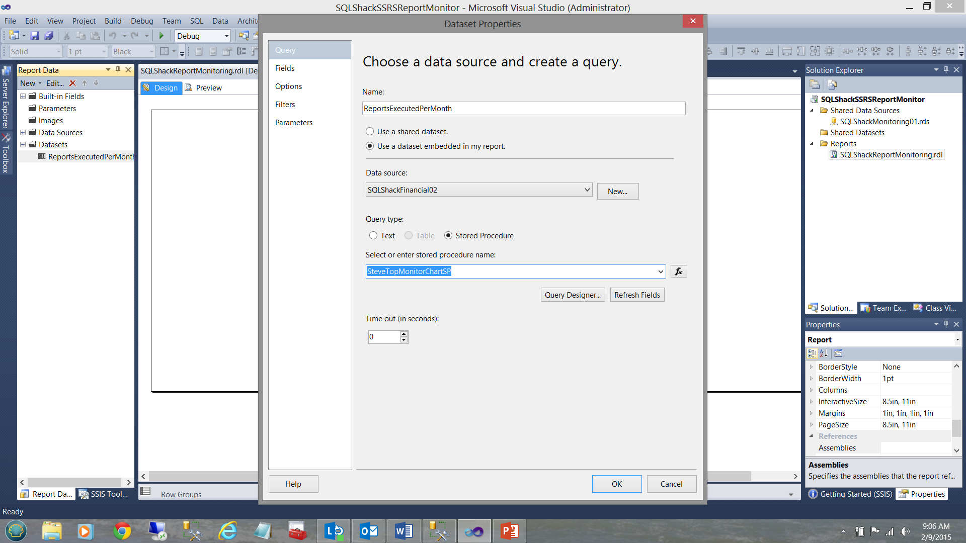
We select the “Stored Procedure” radio button and then click “Refresh Fields” (see above).

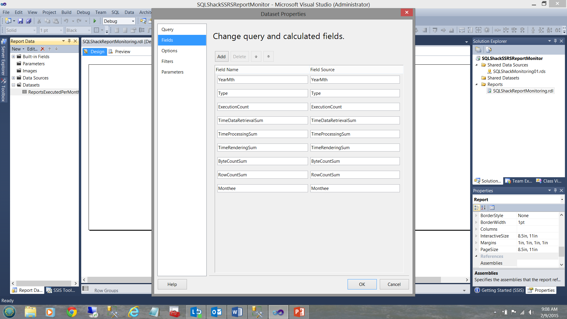
Clicking on the fields tab (see above), we immediately see the fields that we pulled from our first code listing (see Addenda 1). We click OK to exit the “Data Properties” dialogue box.

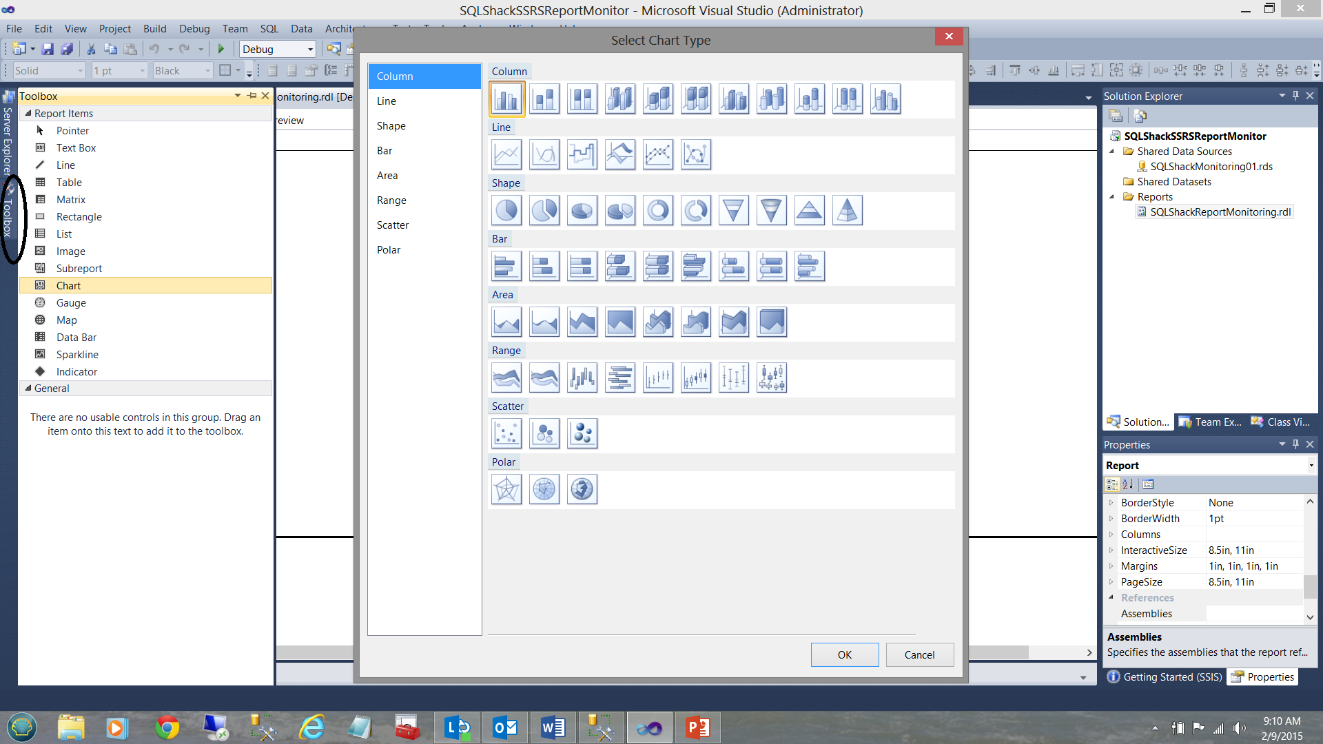
Opening the “Toolbox” (see above and immediately to the left) we add a “Chart” as may be seen below.

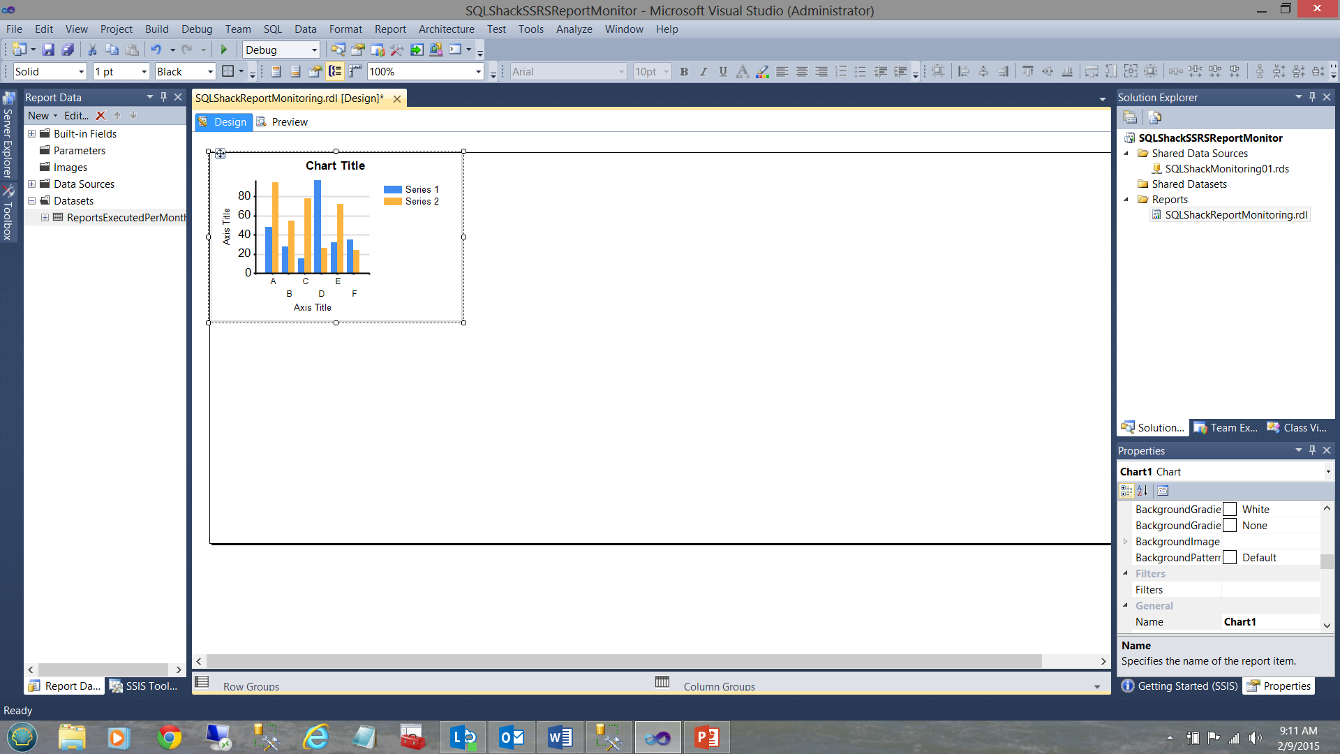
We resize our chart (see below).

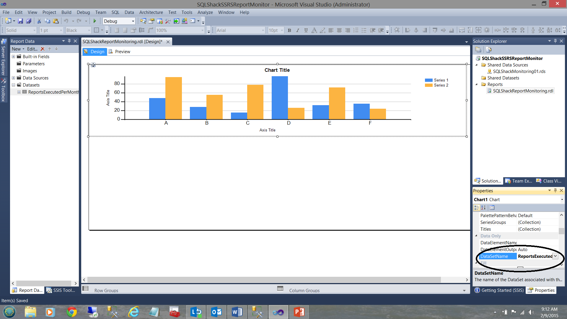
We then set the chart’s “DataSetName” property to the name of the dataset that we just created “ReportsExecutedPerMonth” (see above and to the right).

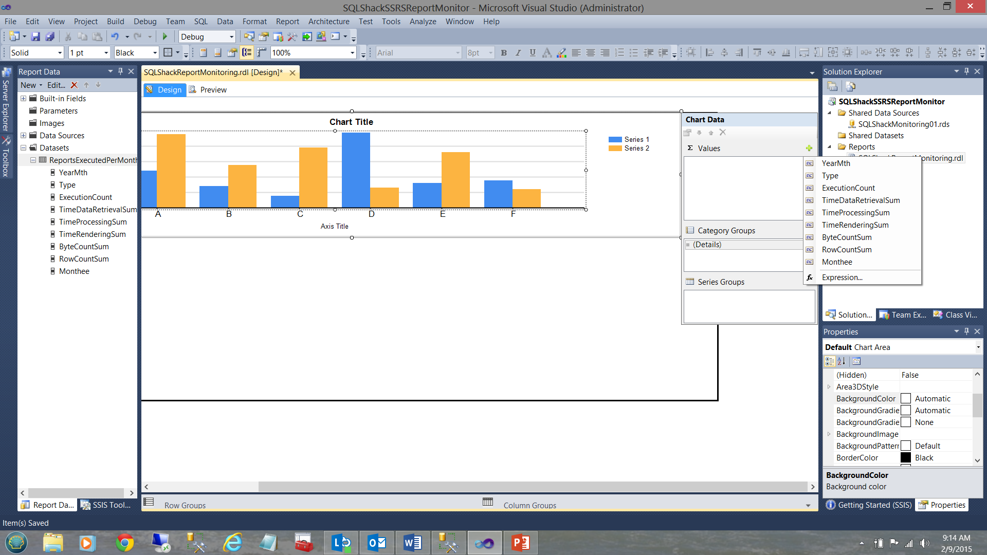
By clicking on one of the columns of the vertical bar chart, we reveal the “Chart Data” dialogue box (see above).

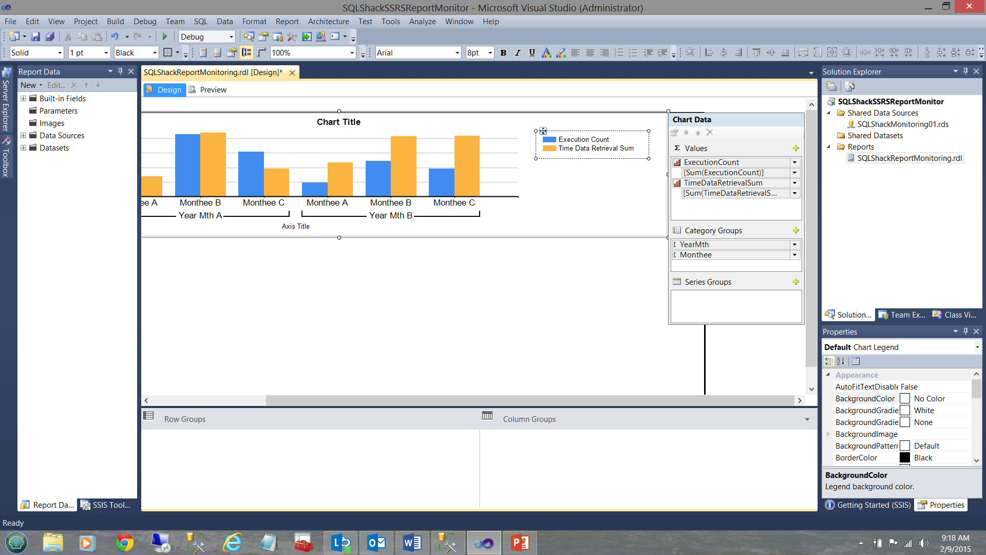
For our “Values” we shall utilize only the “Execution Count” and the “TimeDataRetrievalSum” fields. Obviously, we could have chosen more fields. For the ‘Category Groups”, we select “YearMth” and “Monthee”. The field “YearMth” will ensure that the “Monthee’s” are correctly sorted. We do however have to make one alteration to the “YearMth” field and that is to ensure that it does not appear on our chart. Once again, its sole purpose is to ensure that the months are correctly sorted.

We right-click on the “YearMth” Category Group and select the “Category Group Properties” option.

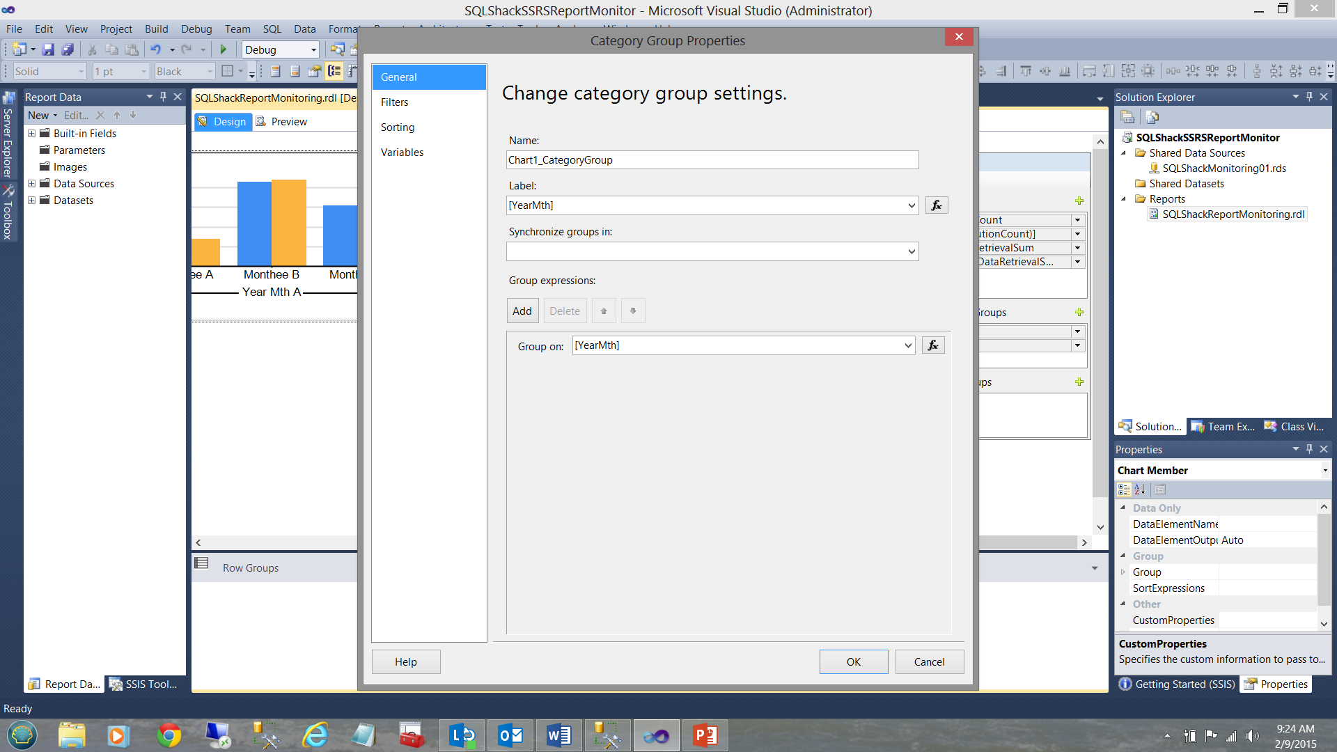
The “Categories Group Properties” dialogue box is brought into view (see above). We click the function box to the right of the ”Label” dialogue box to bring up the “Expression” dialogue box (see below).

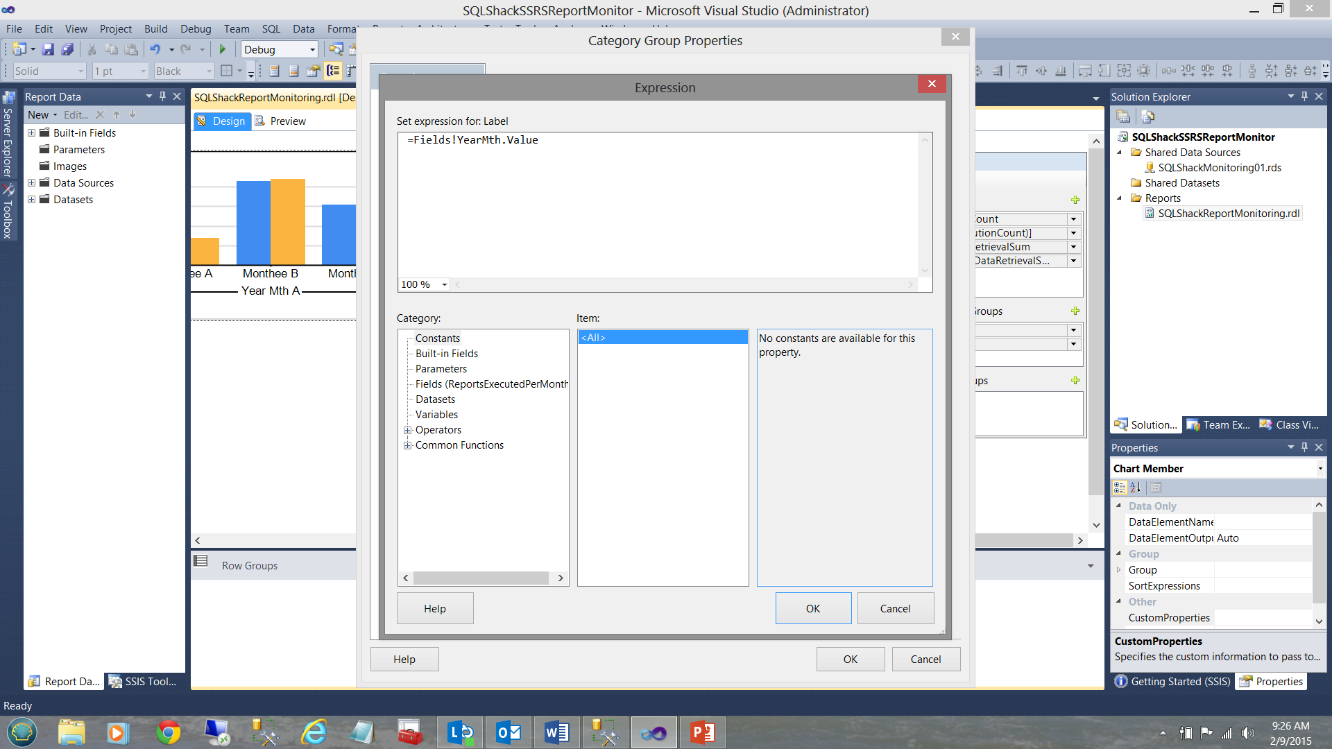
We change the value “ =Fields!YearMth.Value” to “=Nothing” (see below).

We click OK, OK to leave the dialogue boxes.
Let us now see what our report looks like thus far. We click the “Preview” button from our work space ribbon.

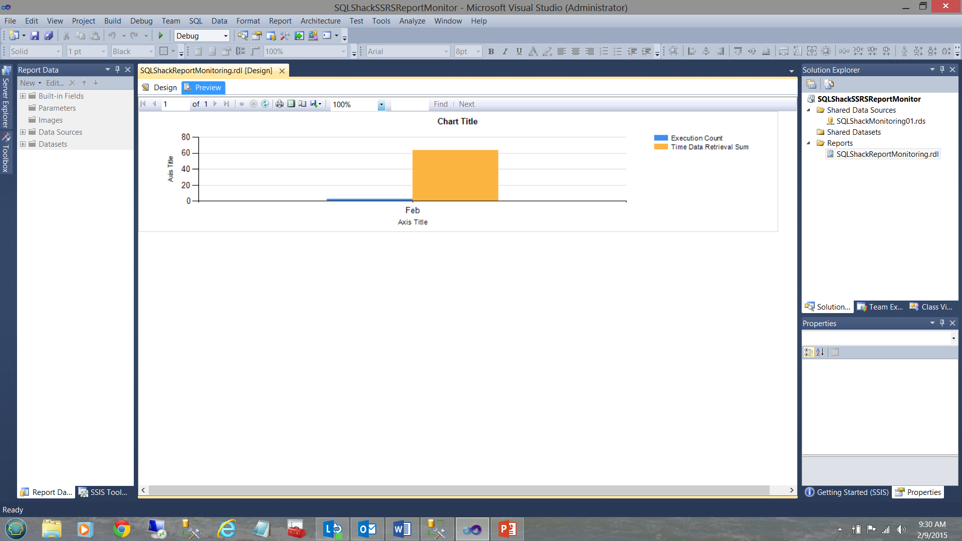
We see our chart for February. Note that the total retrieval time is +/- 60 msec and 3 executions occurred.

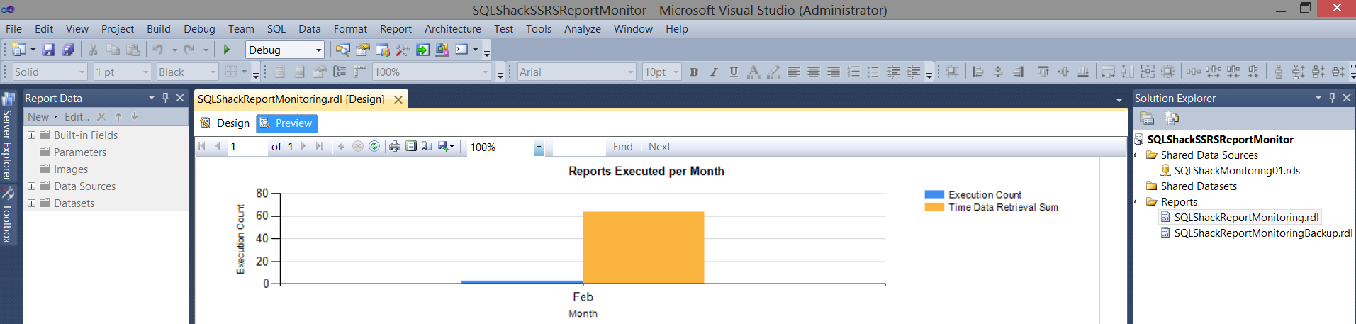
Cleaning our report a tad, we add a title for the chart and label the X and Y axes (see above).

Our chart is a bit simplistic and it would be most useful to have a look at many of the statistics behind the data.

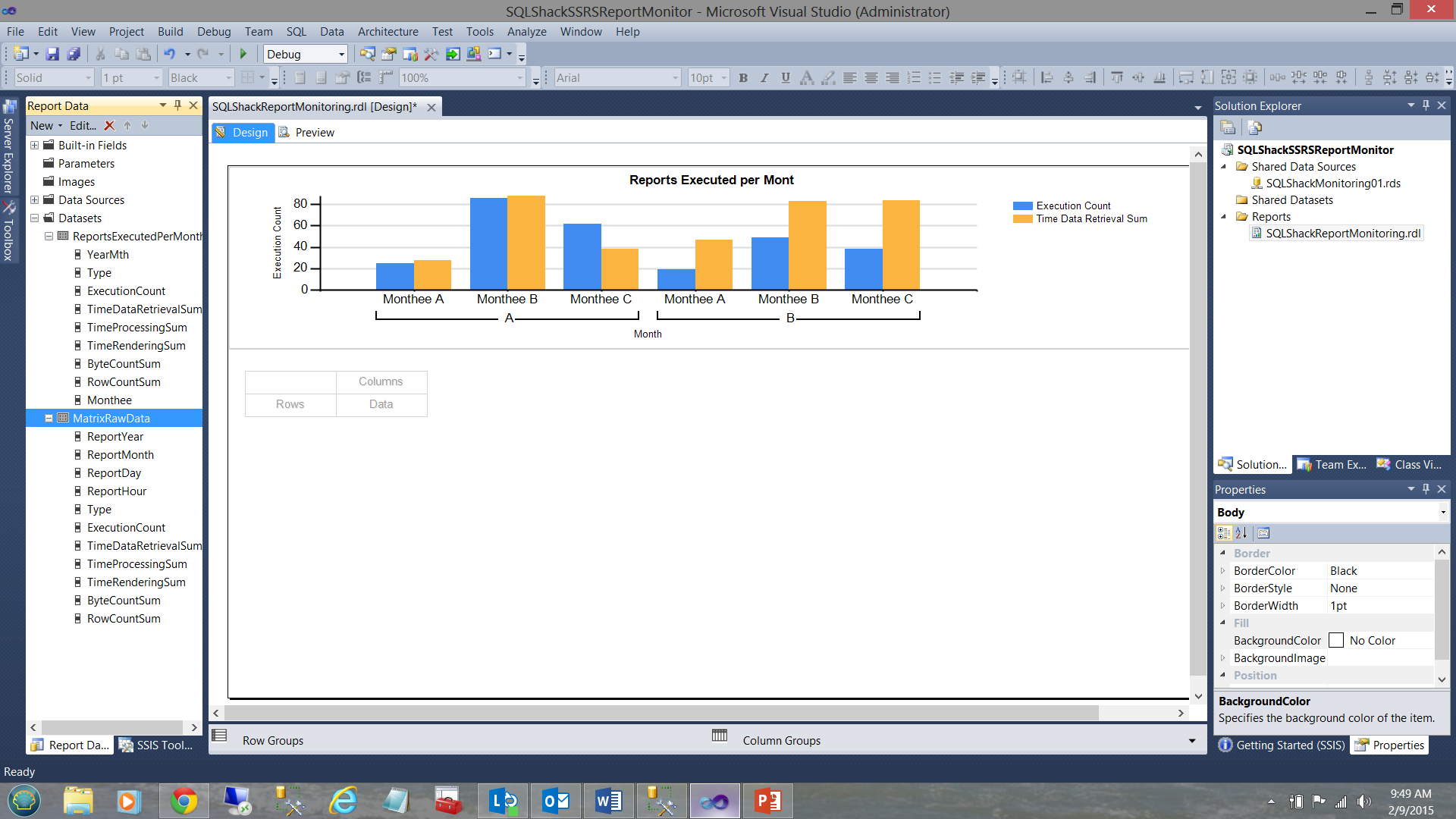
We now add a “Matrix” component below our chart.

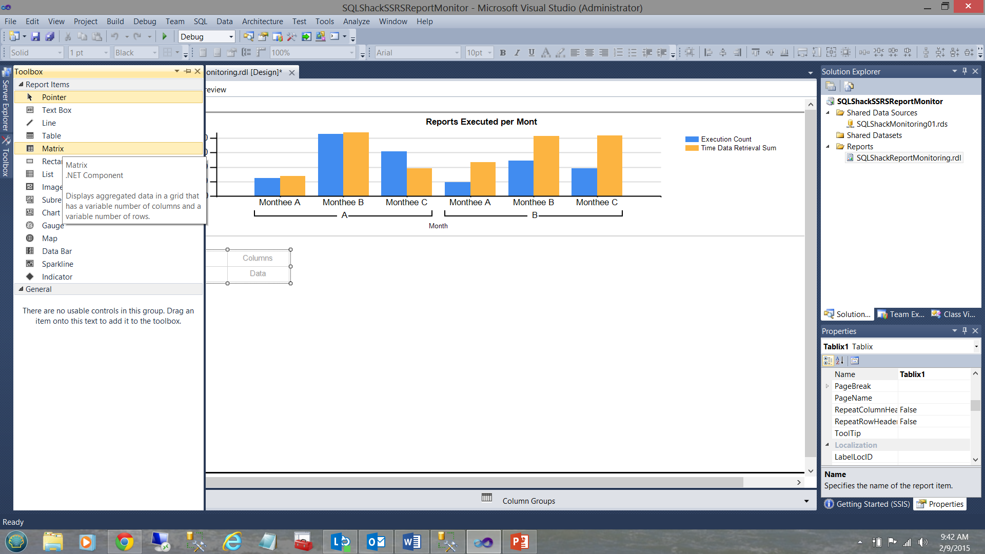
As with the “Chart”, we need to define a dataset with will provide the raw data to the matrix.

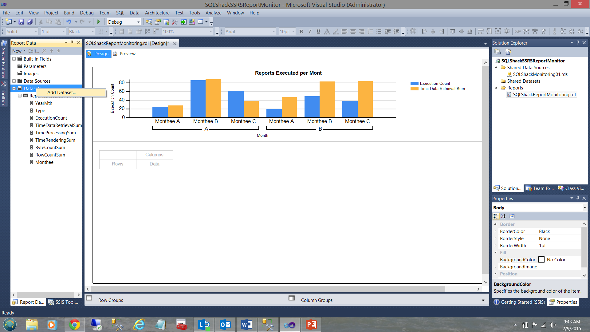
Once again we right click upon the “Dataset” folder and select “Add Dataset” (see above).

We give our dataset a name “MatrixRawData” and select the “Data source” that we created for our chart. Once created, the local data source “SQLShackFinancial02” is available to be utilized for any other local / embedded datasets that require it.

I select the “SteveTopMonitorSP” stored procedure as my data conduit from the database table to the report dataset (see above). We click OK and are returned to our work surface.

The newly created dataset may be seen in the screen dump above.

Clicking upon the matrix, we may now set its “DataSetName” property to our newly created dataset (see below).

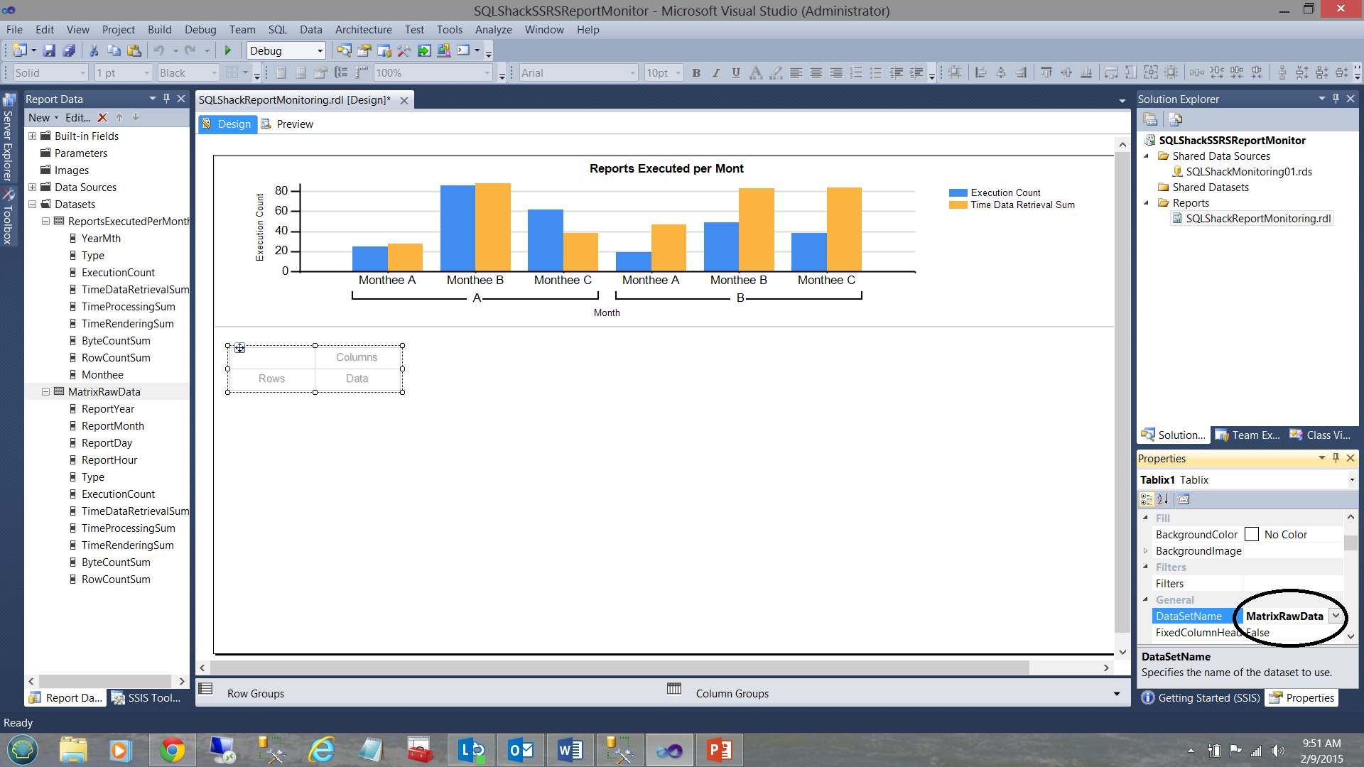
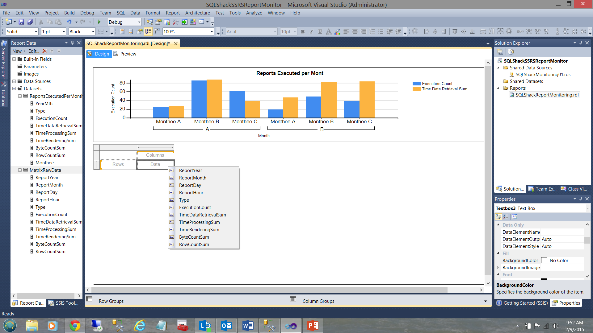
We now note that numerous interesting data fields are available to our Matrix (see below). The code listing providing this data may be seen in Addenda 2.

The astute reader will note that we have a column grouping aspect which may be seen in the screen dump above. We do not require this and therefore we shall now remove the column grouping PRIOR to adding any of the available data fields to our matrix.

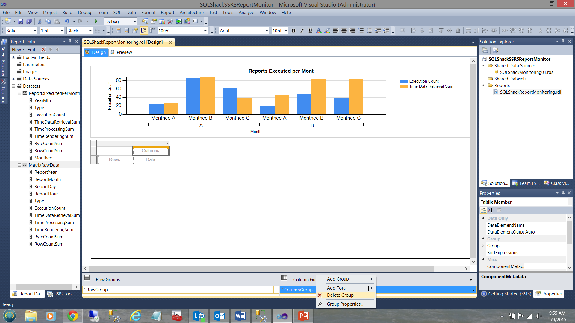
We right click on the “ColumnGroup” and select “Delete Group” (see above).

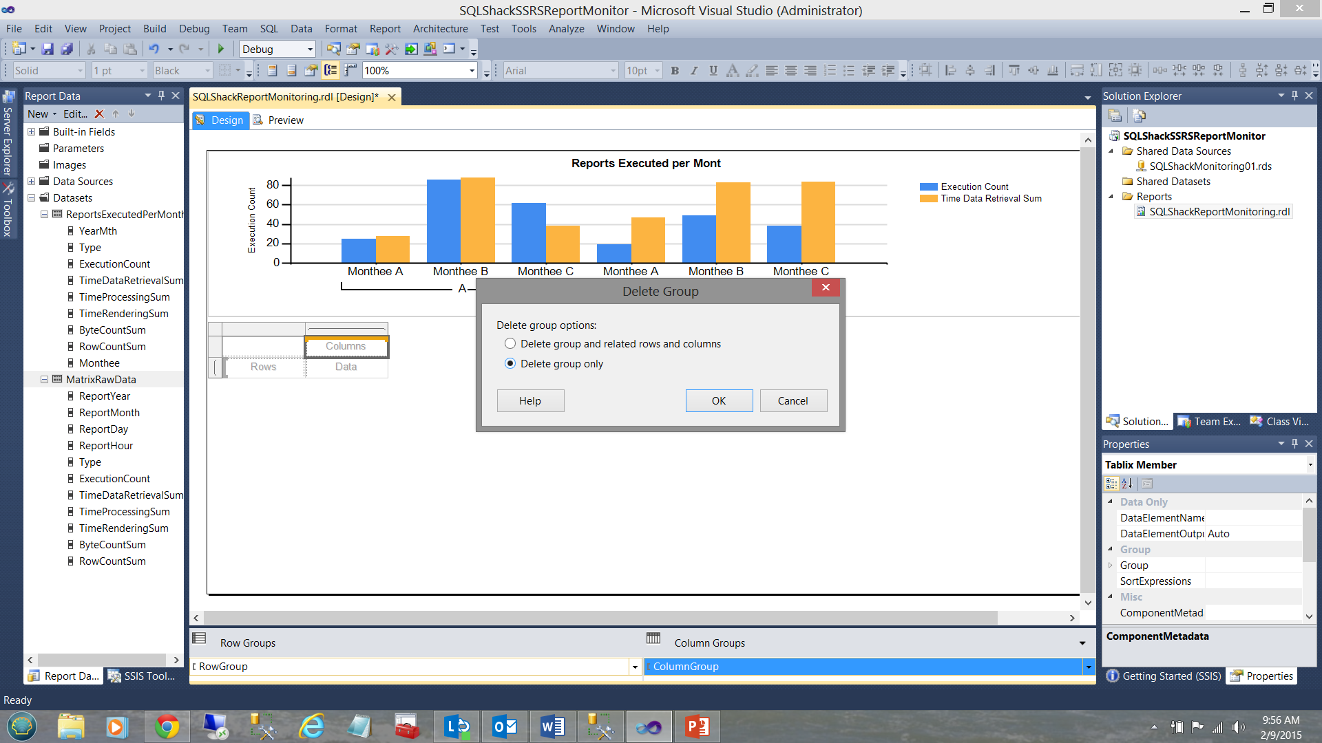
We are asked if we want to delete the data and the grouping OR just the grouping. We select “Delete group only” and click OK.

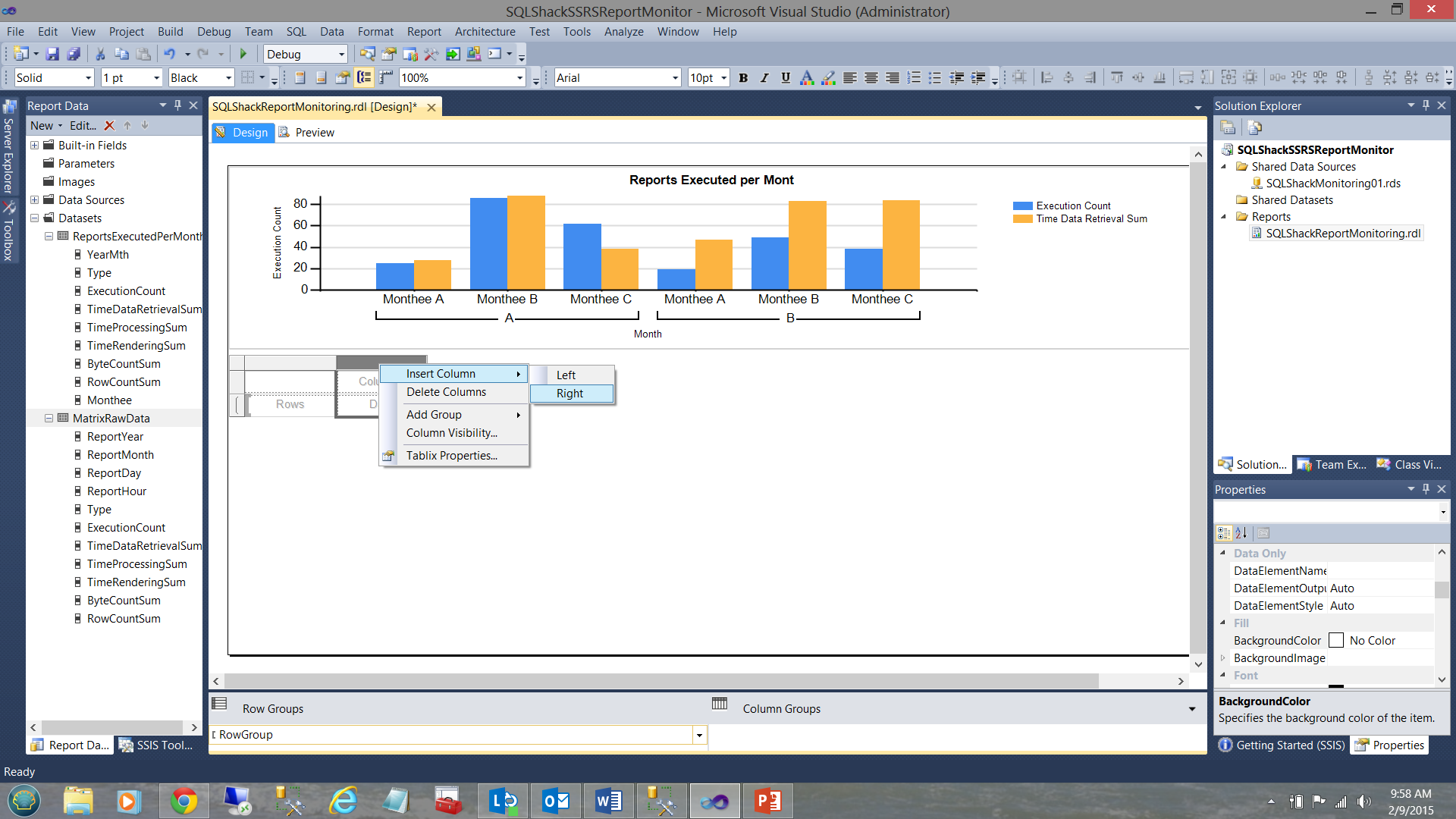
As we have eleven fields that we wish to display in our matrix, we shall add nine more columns to the right of the two columns that we were given when we added the matrix to our work surface.

Our modified matrix (with the extra columns) may be seen above.

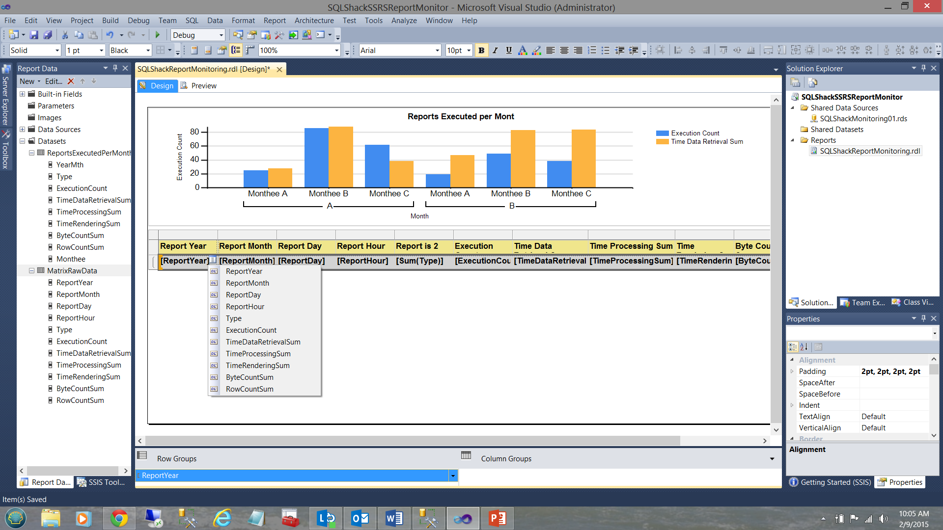
Clicking on the ellipsis in the second row of the matrix (which I have highlighted in grey) we can see the fields that are available to us. Further, I have taken the liberty of populating the fields of the matrix to reflect our needs.

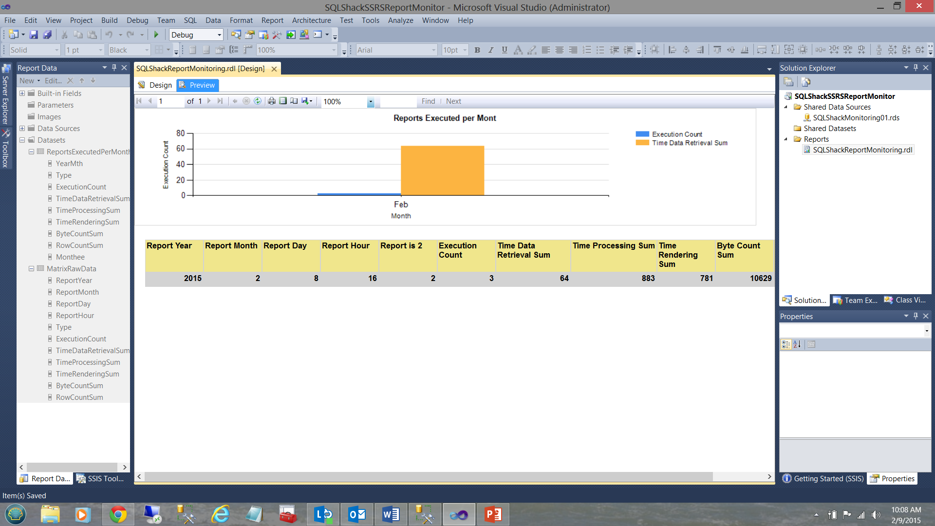
When run, our report now appears as follows (see below).

In a similar manner

In a similar manner, we may add the remaining two matrices that will complete our report and hook them up to the code listings in Addenda 3 and Addenda 4.

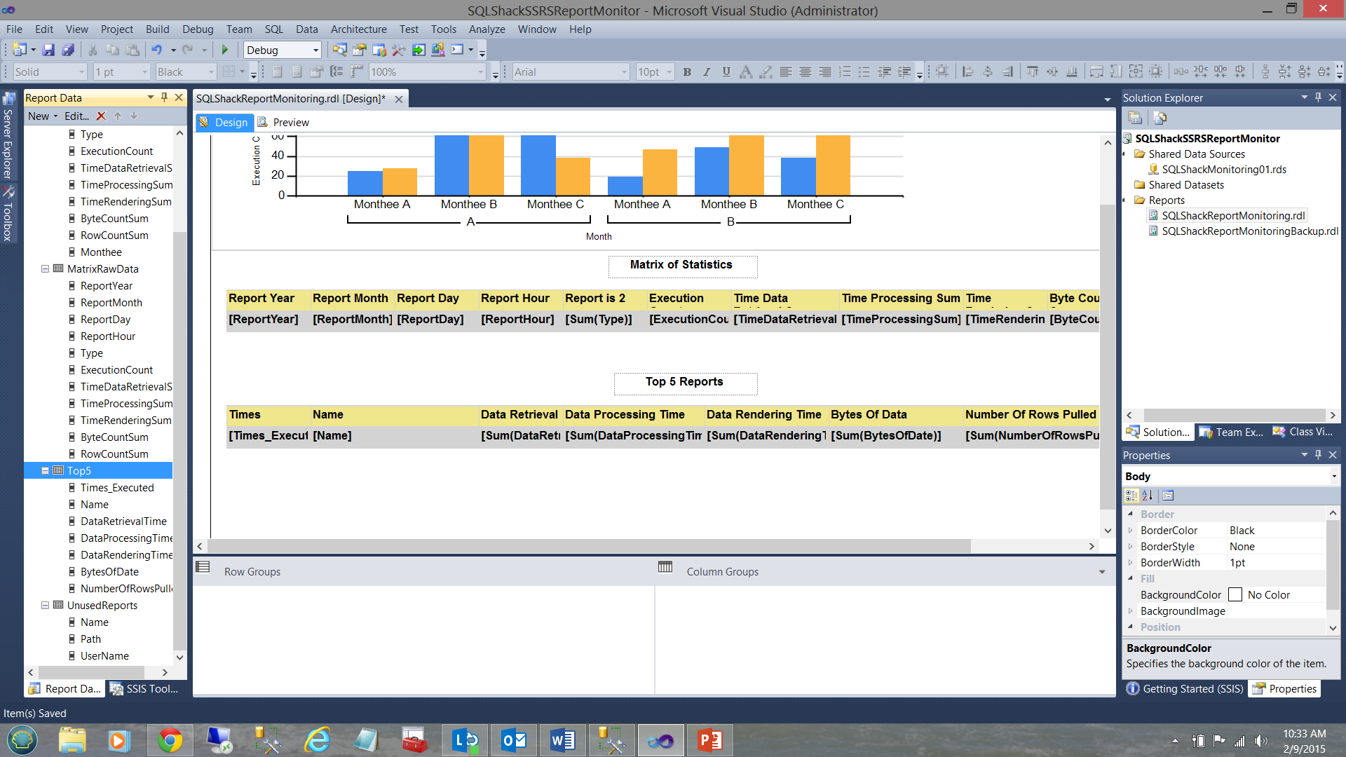
The dataset and matrix for the “Top 5” may be seen above.

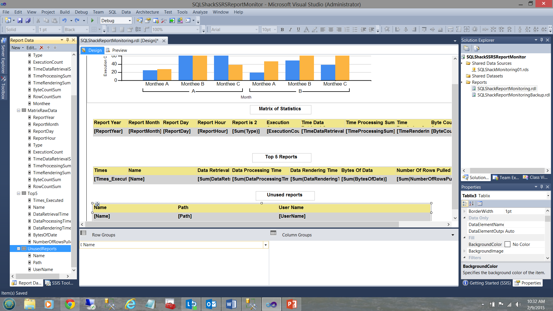
The dataset and matrix for the “Unused reports” may be seen above.

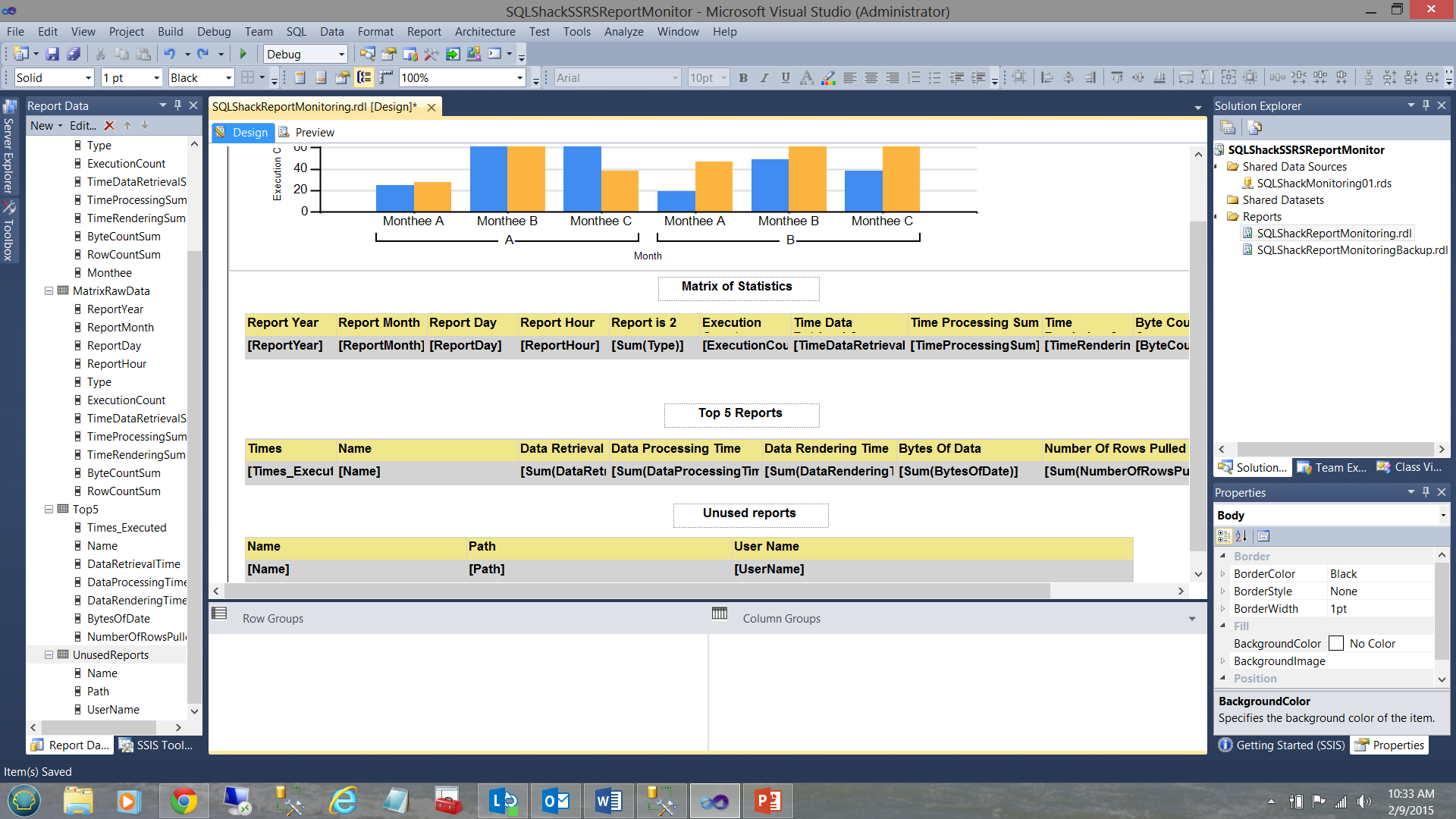
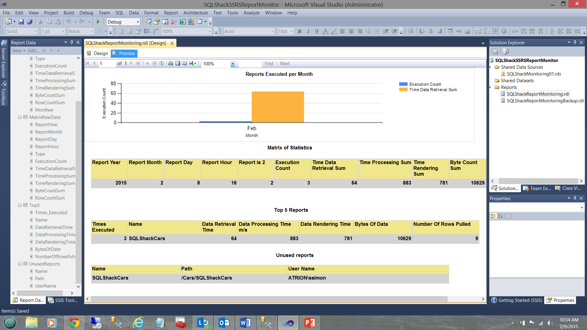
Our completed report may be seen above. Clicking the “Preview” button on the report ribbon, we may see our report results.

Conclusions

SQL Server Reporting Servers often become clogged with reports of minimal importance and /or minimal usage. Regular maintenance and good house cleaning help us ensure that our servers are being both efficient and effective.

Developing a quick and dirty Reporting Services monitor can help us keep our finger on the pulse and inform us of end-user utilization.

The SQL Server Reporting Services database has a wealth of valuable metrics with which to perform our analysis. The “catalog” table contains many of the criteria that we have utilized above.

Whilst we have only touched upon a few of the plethora of available fields, we have amazing possibilities of adding more charts and matrices to our monitoring tool.

Happy programming!!

Addenda 1

Addenda 2 “Report run time statistics”

Addenda 3 “Top 5 Reports”

Addenda 4

• Author
• Recent Posts

Steve Simon

Steve Simon is a SQL Server MVP and a senior BI Development Engineer with Atrion Networking. He has been involved with database design and analysis for over 29 years.

Steve has presented papers at 8 PASS Summits and one at PASS Europe 2009 and 2010. He has recently presented a Master Data Services presentation at the PASS Amsterdam Rally.

Steve has presented 5 papers at the Information Builders' Summits. He is a PASS regional mentor.

View all posts by Steve Simon

Latest posts by Steve Simon (see all)

• Reporting in SQL Server – Using calculated Expressions within reports - December 19, 2016
• How to use Expressions within SQL Server Reporting Services to create efficient reports - December 9, 2016
• How to use SQL Server Data Quality Services to ensure the correct aggregation of data - November 9, 2016