
Introduction
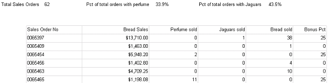
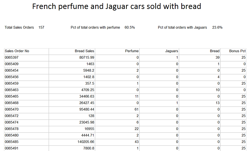
Late in October, I received an unusual request from the head of sales within one of my client sites. Sales sells three articles: bread, perfume, and Jaguar motor cars. Now the reader will note that one of these items is a staple and the other two are for those folks with considerable disposable income. Management within the firm had increased the salesmen’s bonuses for those folks that managed to sell perfume and/or Jaguars along with the standard loaves of bread. The summary report may be seen below showing the final bonus rate for each sales order booked during the month.
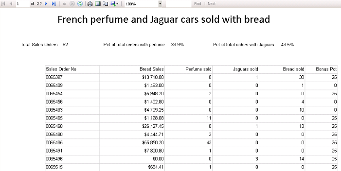
With the scenario now understood, in today’s “fire side chat”, we going to look at how to assemble the necessary infrastructure and learn how to create the report shown above.
Let’s get started!
Getting started
We begin by examining the new business rules. Should a salesperson sell units of perfume and one or more Jaguars, then he or she is entitled to a 40 % commission/bonus on all sales. Further, if he or she only manages to sell one of the product (excluding bread) then the percentage commission is only 25 % on the total sales. If the salespersons sells neither of the products, then there is no commission for the month.
We can code these conditions as follows.
|
1 2 3 4 5 6 7 |
=Switch ( Fields!Perfume.Value > 0 and Fields!Jaguars.Value > 0 , 40 , Fields!Perfume.Value > 0 and Fields!Jaguars.Value=0, 25, Fields!Perfume.Value =0 and Fields!Jaguars.Value>0, 25, true,0) |
and this expression is the main building block of today’s discussion.
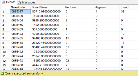
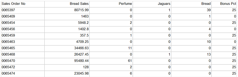
A quick look at the raw data

Having a look at our raw data (see above), we note that the “Sales Order Number” is shown along with the dollar value of the bread sales, the number of perfume units sold, the number of Jaguar cars sold and finally the number of loaves of bread sold. This is the data that we shall be utilizing for our reporting.
The query behind the data may be seen below:
|
1 2 3 4 5 6 7 8 9 10 11 12 13 14 15 16 |
use SQLShack go Create Procedure BigBonus as SELECT [SalesOrderNo] ,[Bread Sales] ,[Perfume] ,[Jaguars] ,[Bread] ,[TotalOrderCount] ,[PerfumeTot] ,[JaguarTot] ,[Breadtot] FROM [SQLShack].[dbo].[Bonus] |
Using this code we create a stored procedure as may be seen above.
Creating our report
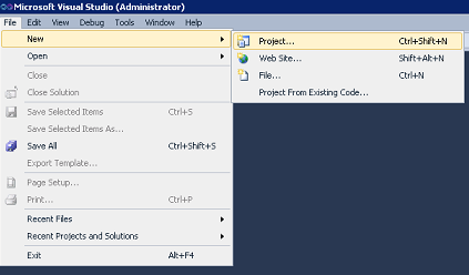
Opening Visual Studio Data Tools 2010 or greater, we create a new project (see above).
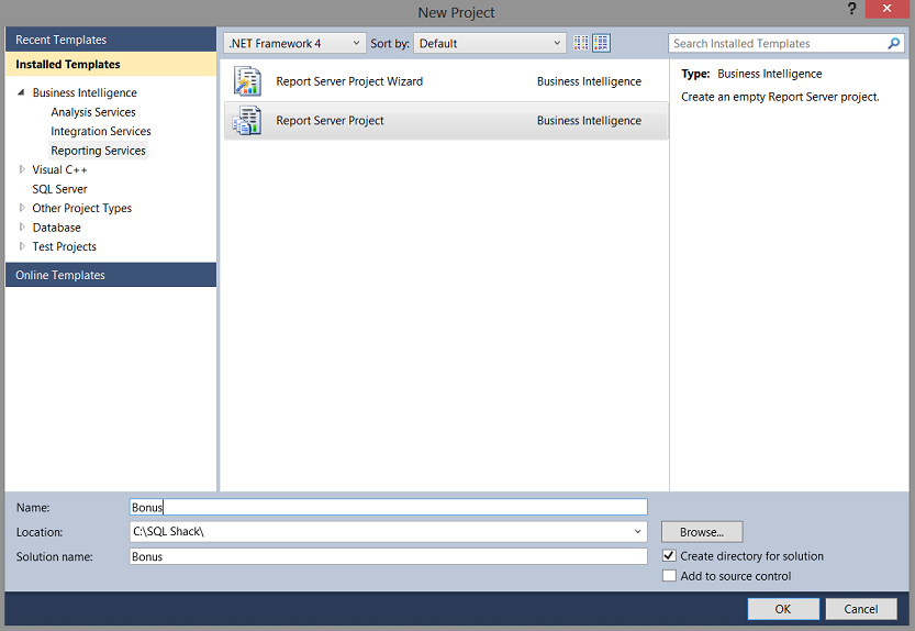
We select the “Reporting Services” project type (see above) and give our project a name. We click “OK to continue.
Connecting to the database to retrieve our data
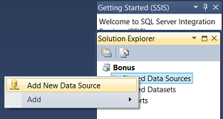
Our first task is to create a connection to our SQLShack database. As in past “get togethers”, I prefer to liken a connection or “Shared Data Source” to a water faucet on the wall of a house. It is the point of entry into the database.
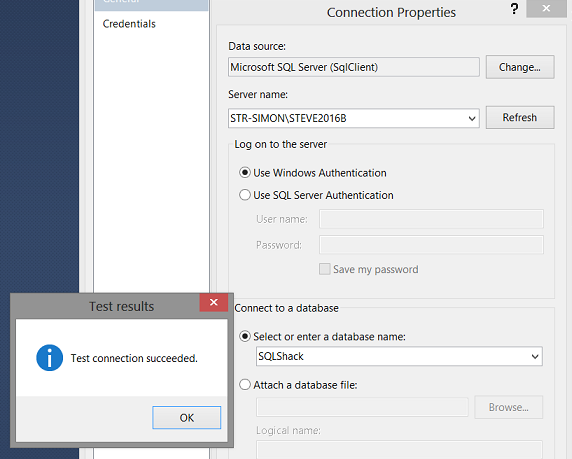
We set the connection to point to the SQLSHACK database and test the connection (see above). We click “OK” and “OK” to leave the “Shared Data Source” / connection dialog box.
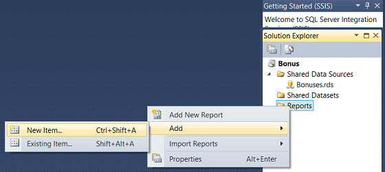
Our next task is to create our Report. We right click on the ‘Reports” folder (see above) and select “Add”, and “New Item” from the context menu (see above).
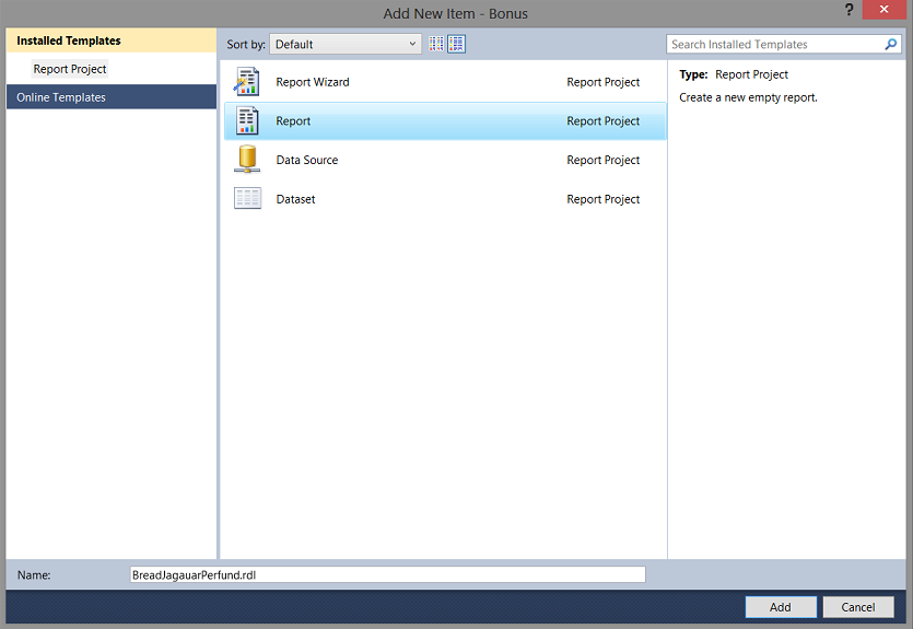
We find ourselves on the “Add new Item” page. We select “Report” and give our report a name (see above).
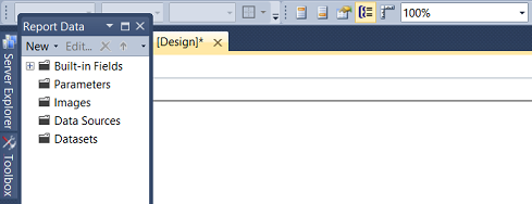
We find ourselves on the report drawing surface (see above).
Our next task is to create a local dataset.
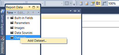
By “right clicking” on the dataset tab (see above), we bring up the context menu and select “Add Dataset”.
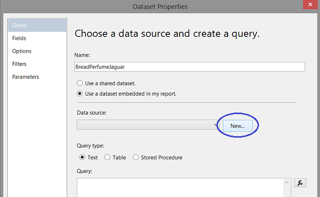
We give our dataset a name and select “Use a dataset embedded in my report” (see above). This achieved, we must create a new “Local Data Source” to access the “Shared Data Source” and this “Shared Data Source” accesses the stored procedure that we created above.
As I have often mentioned in past “fire side chats”, I prefer to work with local data sources and local data sets as they permit local refining of selection criteria both from a data point of view and additionally increased flexibility with query predicates. We click the “New” button to create a new local data source (see above).
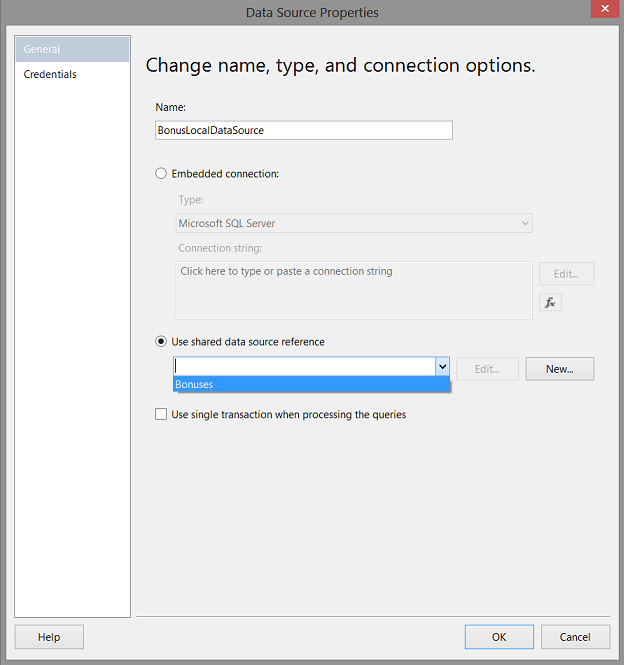
Having clicked the “New” (local data source) button (as discussed above), we find ourselves on the “Data Source Properties” page. We give our local data source a name and point this local data source to the “Shared Data Source” that we created above. In short, our local data source will “connect up” with the “Shared Data Source” and will tap off of the data retrieved via the “Shared Data Source”. We click “OK” to continue.
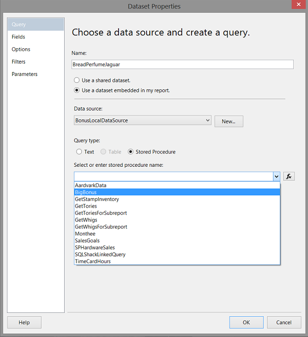
We find ourselves back upon the “Dataset Properties” screen. We toggle the “Stored Procedure” radio button and select the “BigBonus” stored procedure (see above).
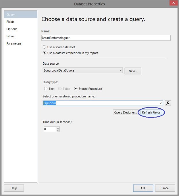
Having selected the stored procedure, we click the “Refresh Fields” button to pull the database table field names that will make up the structure of the data set.
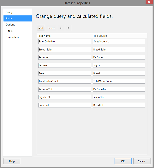
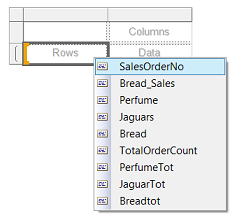
Having “clicked” the “Refresh Fields” button and THEN clicking the “Fields” tab (see above and to the left), we note the structure of the dataset (see above).
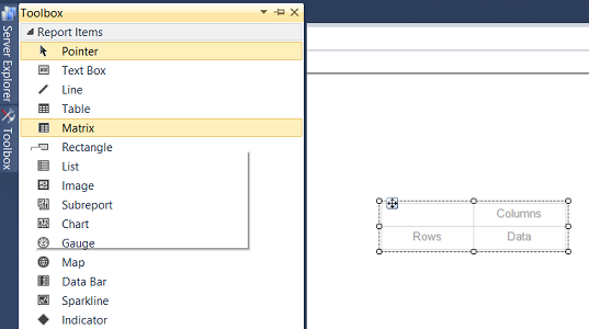
Now that our dataset has been created, our next task is to drag a “Matrix” control (from the toolbox) onto the “Design Surface” as may be seen above.
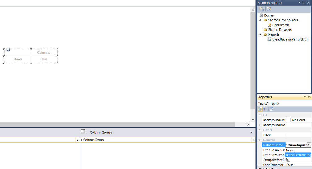
Highlighting the matrix that we just added and by pressing F4, we activate the properties menu. We set the dataset name property of the matrix to the name of the dataset that we just created. By doing so we define the fields that will be available to the matrix (see above and to the bottom right).
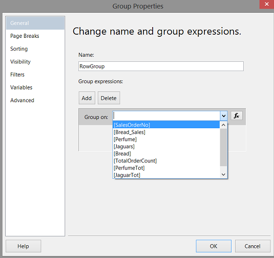
Now that our “Matrix” has been correctly configured, our next task is to define our summary grouping field. We right click on the “RowGroup” tab (see above) and set the “Group on” field to “SalesOrderNo” as shown above. In other words “Sum the units sold by the sales order number”.
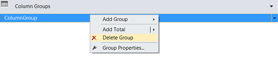
As we do NOT require the column grouping, we right click on the “ColumnGroup” tab (see above). We select “Delete Group” (see above).
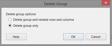
We are now asked whether we wish to “Delete group and related rows and columns” or rather to just “Delete group only”. We select “Delete group only” (see above).
Adding data columns to the matrix
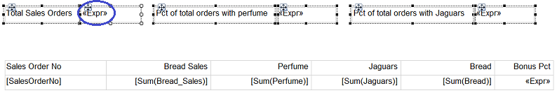
We add our grouping column “SalesOrderNo” (see above) and then the “Bread_Sales”, ”Perfume”, ”Jaguars” and “Bread” fields (see below). In a few moments, we shall see how to utilize the remaining fields within the dataset.

Calculating our Commission
We are now in a position to add another field to the matrix, however, this time this field will be a calculated field. The astute read will remember that should a salesperson have sold both Jaguars and Perfume, then he or she is entitled to a 40 % commission. If he or she was able to sell one or the other of the high ticket priced items then the commission is 25 %; otherwise, no commission is paid.
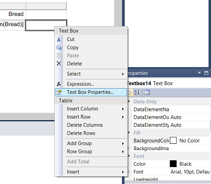
This said, we add a “Bonus Pct” column and bring up the “Text Box Properties” option from the context menu. The context menu is brought into view by “right clicking” on the text box as may be seen above.

The “Text Box Properties” dialogue box opens. We click the “Value” function button to open the “Expression” dialogue box (see above).
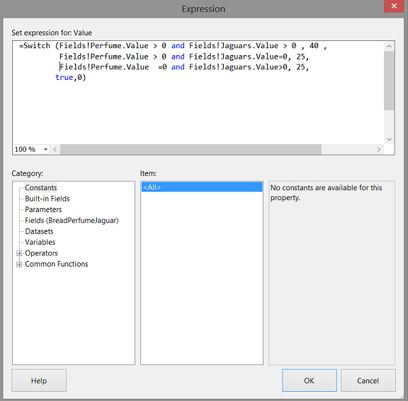
Finally we add the code snippet that we encountered at the beginning of our “get together”. This code merely applies the commission/bonus calculation rules. We click “OK” to continue.

Our matrix now appears as follows. Note the “Commission” field.
Running the report shows us the application of the business rule (see above).
Adding the bangers and whistles
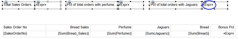
Our last task is to add the summary line calculations for the “Total Sales Orders”, the “Pct of total order with perfume” and the “Pct of total orders with Jaguars” (see above).
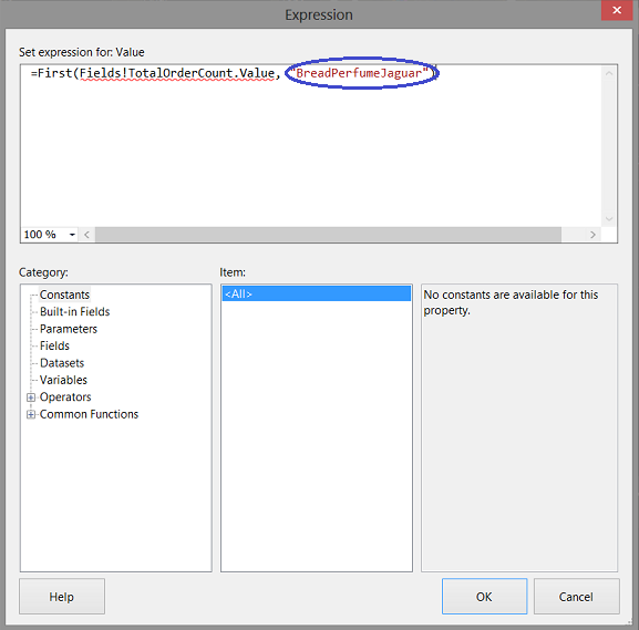
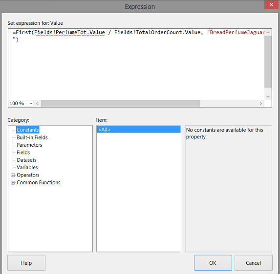
We first create the expression to display the total number of sales orders (see above). The astute reader will note the word “BreadPerfumeJaguar” in red. This is the name of the local data set that we created above.
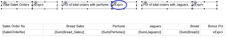
We now configure the sales percentage of perfume (see above).
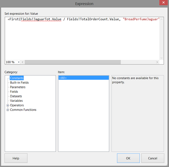
Finally we configure the sales percentage of Jaguar sales (see above).
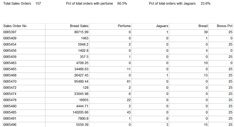
Our completed report may be seen above and as the last addition, we add a title to the report (see below).
Thus our report is now complete and ready to go and our task is now complete.
Conclusions
Most of us from time to time have been requested to produce challenging summary level reports. Whilst the report that we have just created is somewhat simplistic, the one takeaway is the power of utilizing calculated expressions within our reports. These expressions provide flexibility and allow for changing conditions within the business environment.
Until our next “get together” happy programming and the best for the upcoming festive season!
Steve has presented papers at 8 PASS Summits and one at PASS Europe 2009 and 2010. He has recently presented a Master Data Services presentation at the PASS Amsterdam Rally.
Steve has presented 5 papers at the Information Builders' Summits. He is a PASS regional mentor.
View all posts by Steve Simon
- Reporting in SQL Server – Using calculated Expressions within reports - December 19, 2016
- How to use Expressions within SQL Server Reporting Services to create efficient reports - December 9, 2016
- How to use SQL Server Data Quality Services to ensure the correct aggregation of data - November 9, 2016