
Partitioning is the concept where you divide your data from one logical unit into separate physical chunks. This can have several advantages, such as improved performance or easier maintenance. You can for example partition a table in a SQL Server database, but you can also partition your measure groups inside an Analysis Services (SSAS) Multidimensional cube. In this article, we’ll discuss how you can set-up partitioning. For more information about the expected benefits, take a look at Benefits of Partitioning your SSAS Multidimensional Cube.
Note that you can also partition tables in Analysis Services Tabular. Although similar in concept on a high-level, we’ll keep the focus of this article on Multidimensional only.
Test set-up
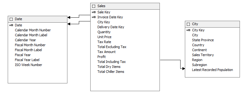
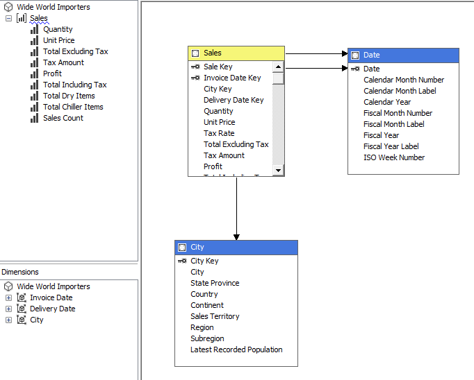
In this article we’ll use the free sample database Wide World Importers Data Warehouse, which you can find on Github. I’ve imported three tables into the Data Source View: Sales (Fact table), Date and City (two dimensions).
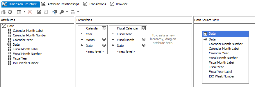
The Date dimension has the following structure:
The following attribute relationships are defined:
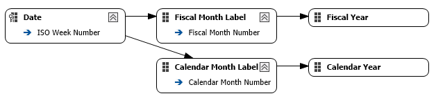
Since we don’t expect the calendar to change in format any time soon, all the relationships are defined as Rigid.
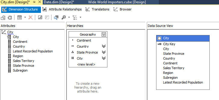
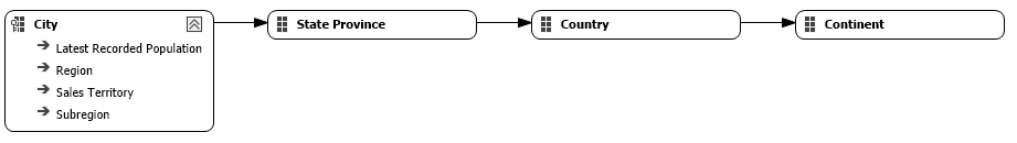
The City dimension has the following structure:
There are also attribute relationships defined and because continents usually don’t change that much they are defined as Rigid as well.
The cube itself is simple: one measure group with all measures from the Sales fact table (except the Tax Rate measure), linked with our two dimensions.
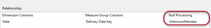
One important detail: the foreign key Delivery Date Key from the Sales table to the Date dimension might contain null values, so we set the Null Processing property to UnknownMember. If you don’t set this property, the cube will fail during processing.
In theory, the cube is finished. You can deploy it to a server, process it and analyze the data with your favorite front-end tool.
Creating Partitions
Typically, partitions on a measure group are based on a time column. This makes sense, as it is a natural way of partitioning data: every day new data comes in and all time boundaries are clearly defined. Partitioning on time also allows you to partition on different levels: old data can for example be put in yearly partitions, while new data can be partitioned at the month level or even at the day level. Most examples you can find online are based on time partitioning. In this article, we’re going to look at a different angle: we are going to partition the measure group on Sales Territories. There are two possible reasons for making this choice:
- Sales Territories are relatively fixed. Normally, they aren’t any new ones created daily. This means that you can define your partitions once and they don’t need much maintenance afterwards. With time partitions, you need constant maintenance to create new partitions or to merge older partitions together. Typically, you’d solve this by automating your partition management.
- Later, we might want to add security on top of our Sales Territories. In other words, some users might only see data for a specific sales territory. Partitioning on those territories might give additional performance benefits.
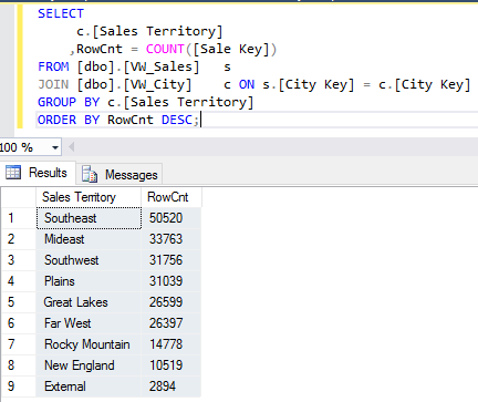
With the following query, we can identity our potential partitions and their size:
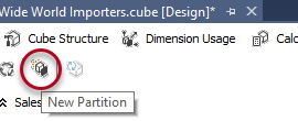
To start creating partitions, we need to go to the Partitions tab in the cube editor.
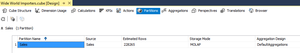
There is a default partition that will contain all the data for the measure group. I already created an aggregation design and assigned it to the partition.
When you click on the Source, you can configure where the partition fetches its data from. The default is Table Binding.
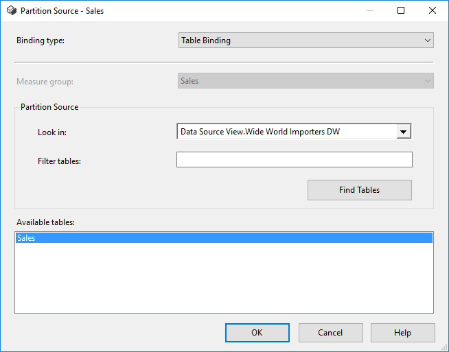
With Table Binding, you select all the data from a certain table. The other option is to use Query Binding, where you can specify the query yourself that fetches the data.
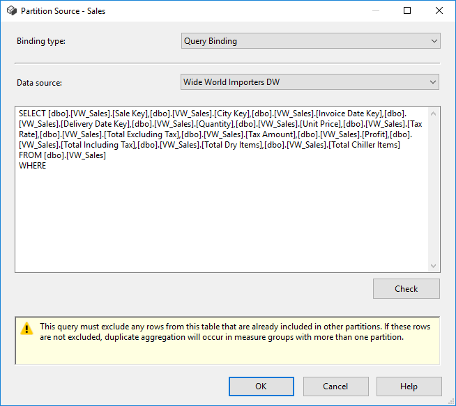
You either have the choice to partition the data at the source with Table Binding – by using different views on top of a table for example – or by specifying different queries for each partition. With the first option, you might clutter your data source view with a lot of additional tables. Query binding is the easiest option and lends itself nicely for automatic partition creating.
Let’s specify the query for our first partition: The Southeast sales territory.
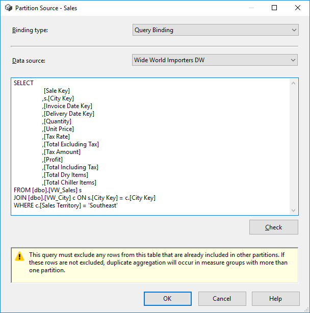
Don’t end your T-SQL statement with a semicolon (although this is the recommendation everywhere else), because this will cause the cube to fail during partition processing, even though the syntax check is successful.
Since we modified the default partition, the partition ID will always be the name of the measure group (Sales), even if we rename the partition to “Sales – Southeast”.
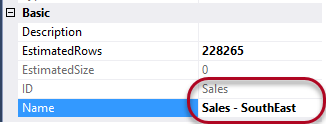
If you want to avoid this, you can create a new partition first and then drop the default partition.
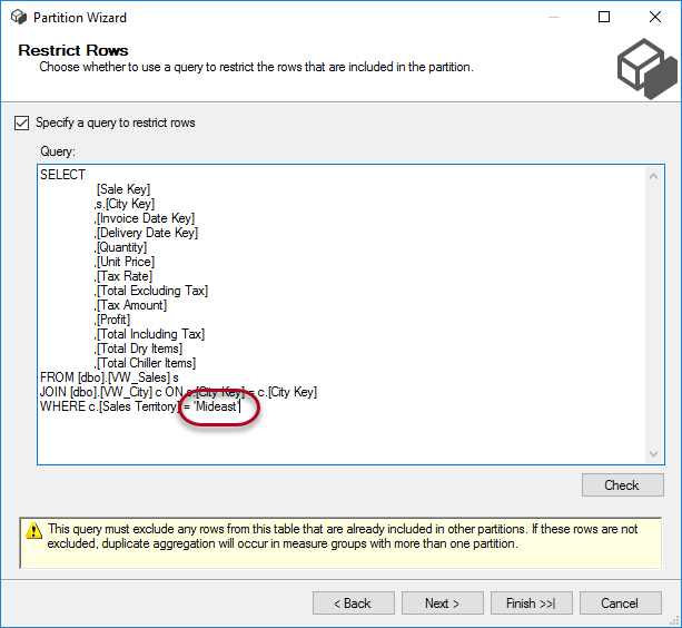
Let’s create a new partition for the Mideast territory.
In the wizard, you’ll first need to select a source table.
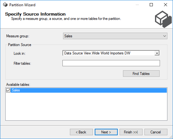
In the next step, we choose to specify a query and enter a modified version of the earlier query:

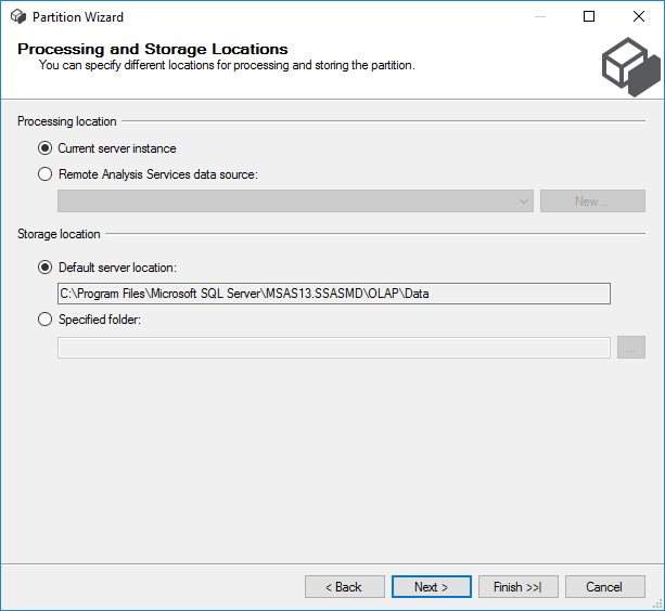
After that, we can choose the storage location of our new partition and we can even configure the partition to be processed at another location. We’re going to leave everything at the default settings. If you want though, you could put partitions at different disks to optimize throughput.
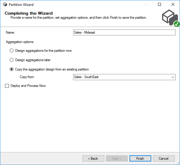
At the final screen, we can configure aggregations – which we’re going to copy from our other partition – and if the partition needs to be deployed and processed right away.
Our partition is ready. You can also change the Storage Mode for a partition. A detailed explanation is out of scope for this article, but these are the high-level concepts:
- MOLAP. The data is read into the model, processed and stored on disk. If there are any aggregations, they are calculated and stored on disk as well.
- ROLAP. The data stays at the source and the model only functions as a metadata layer between a front-end tool and the data source. This storage mode allows for more real-time analysis but might be slower.
- HOLAP. A hybrid combination between the two above.
Similar partitions were created for the other sales territories.
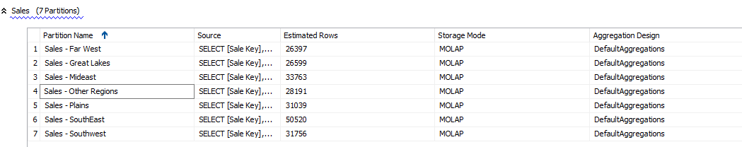
The last three territories – Rocky Mountain, New England and External – and the dummy value N/A are combined into one single partition: Sales – Other Regions. Those territories don’t have enough data to justify a partition on their own, so we combined them into one bigger partition.
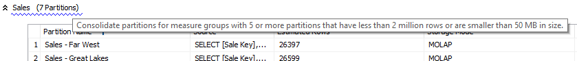
In fact, SSAS warns us that our partitions are too small: SSAS advices to not partition a measure group with less than 2 million rows. However, we are just working with sample data so we can safely ignore this warning.
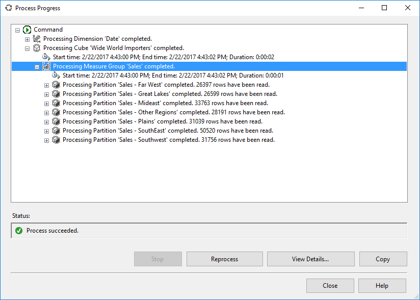
All that is left is to deploy and process the cube.
The article continues with the advantages of partitioning in Benefits of Partitioning your SSAS Multidimensional Cube.
Conclusion
Creating partitions in Analysis Services isn’t a difficult task. In this article, we showed you how you can manually create and configure partitions for a measure group. Your partition strategy defines if you need to set-up partitioning only once – as in the article – or that you continually must create new partitions (for example when you partition on time). If partition maintenance is an ongoing task, you might want to consider to automate it.
The next articles in this series:
- Benefits of Partitioning your SSAS Multidimensional Cube
- How to optimize the dimension security performance using partitioning in SSAS Multidimensional

Koen has over 7 years of experience in developing data warehouses, cubes, and reports using the Microsoft BI stack. Somehow he has developed a particular love for Integration Services along the way.
He has a blog at http://www.sqlkover.com and he is a frequent speaker at local SQL Server events. You can find him on Twitter as @Ko_Ver.
View all posts by Koen Verbeeck