

Introduction
In the article How to partition an SSAS Cube in Analysis Services Multidimensional, we explained how you can partition your measure groups in an SSAS cube. In this article, we’ll look at the expected benefits of the partition strategy. Time to reap the benefits of our hard work.
Partition Benefits
The first benefit becomes clear after we’ve deployed the cube, during processing:
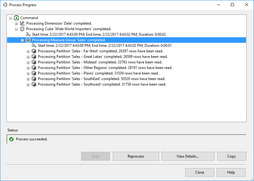
All the partitions can be read and processed in parallel, which maximizes throughput (especially if you saved them on separate disks) and can reduce processing time of your measure group. The amount of processing reduced depends on the number of processors SSAS has available.
There are other benefits related to processing:
- If partitions aren’t updated any more, you don’t need to do a Full Process on them. For example, if you partition on the time dimension and you only add new rows (you don’t update older rows), you only need to do a Full Process on your latest partition. All the other partitions need a Process Index to keep the indexes and aggregates up to date with the latest changes in the dimensions. This can also significantly reduce processing time, because you don’t need to read data from disk for all the older partitions. Keep in mind if you do a Full Process on a dimension, partitions from associated measure groups will be unprocessed. For this set-up to work, the dimensions must all be processed with Process Update.
- You can choose to store older partitions – which are less accessed – using ROLAP and your most recent, frequently accessed partitions using MOLAP. In that case, you only need to process your most recent partitions. There is a performance hit for older partitions, but since they are read less often this might be acceptable.
You can also store your older partitions on cheaper, less faster disks and your most recent partitions on more expensive faster disks (such as SSDs). Processing won’t benefit from this, but it might save you costs on expensive disks if you have a very large cube.
One of the most important benefits however is not related to processing time, but to query performance. When you have defined partitioning and your MDX query only select data from a certain partition, all the other partitions won’t be read. This can significantly reduce your query response time. This is called partition elimination. Let’s look at an example.
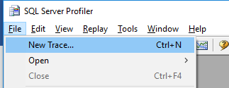
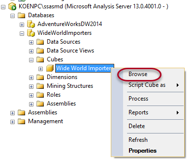
First, we start up profiler so we can monitor the queries sent to the cube, but also find out which partitions are being read from disk. Create a new trace.
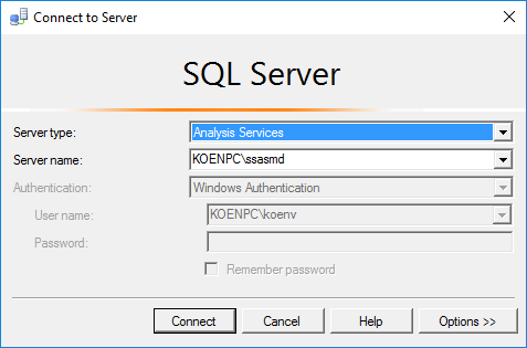
Connect to your SSAS instance.
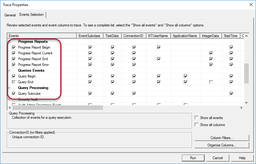
In the Events Selection tab, only keep the events from the sections Progress Reports, Queries Events and Query Subcube selected.
Click Run to start the trace. In Management Studio, we are going to browse the cube to generate some MDX queries.
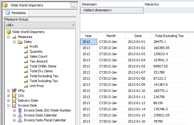
Let’s drag in the Calendar Hierarchy and the Total Excluding Tax measure.
When we take a look at the trace, we can see all the partitions were read:
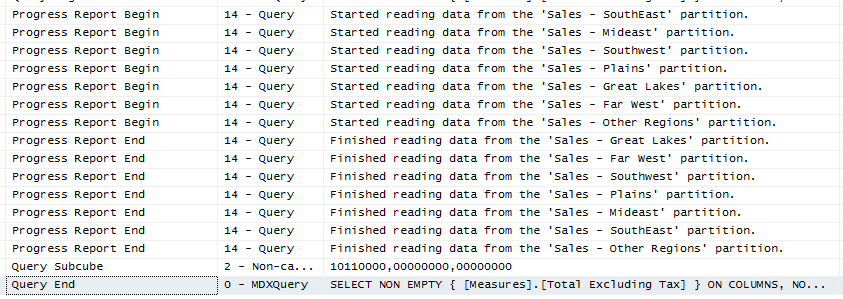
Even though there’s no partition elimination for this particular query, it can already benefit from the parallel execution on the different partitions.
Let’s create a filter using the Sales Territory attribute.
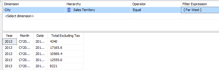
When we look at the Profiler trace, we can now see only one single partition was read:
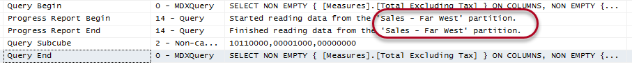
If we would have a very large cube with data evenly distributed over all our 7 partitions, the cost of reading data would be 1/7th of the original query!
Partition Slices
But how does SSAS know which partitions to eliminate? This is done using the partition slice, a property of the partition.
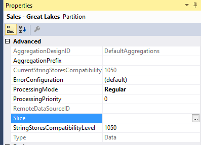
You can set this property manually. For the Far West partition, this would be [City].[Sales Territory].&[Far West]. You can drag and drop the appropriate member to the expression editor:
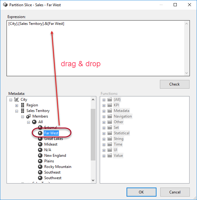
Now SSAS knows the partition only includes data for this particular Sales Territory. For MOLAP storage, SSAS automatically detects which data is loaded into a partition and it will set the slice accordingly (internally, you won’t see a change in the slice property). However, this is not 100% waterproof. For optimal configuration, it’s recommended to set the slices manually.
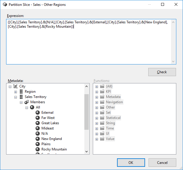
It might be possible for example that SSAS can’t detect which slice to set for the “Others” partition, since it consists of multiple members. In that case, SSAS might set the slice to a higher level of the hierarchy – the ALL member in this case – instead of using OR to join the members together in one slice. This means the partition might be scanned for queries, while the data wasn’t needed after all.
Let’s illustrate with another example: if you have a slice on Q1 and Q2 of 2016, SSAS might create the slice on the lowest common member: the year. If you query the first quarter, a whole year of data might be read.
For the “Others” partition, we can set the slice using a set expression:
We can verify it works when we set the filter to Rocky Mountain and External:

There are several reasons why partition elimination might not always work as you’d expect. Many-to-many relationships might for example prevent that partitions are eliminated if the partitions are defined on the intermediate dimension. Chris Webb explains this in the blog post Many-to-Many Relationships and Partition Slices.
Another issue might arise if you use an attribute that has multiple columns as its key attribute. Suppose you have a YearMonth attribute, where the key columns are defined by a Year attribute and a Month attribute. The order in which you specify the key columns might have an impact on how internally the data is structured. If you specify the month first and then the year, the data might be structured as follows:
Month 1 Year 1, Month 1 Year 2, Month 1 Year 3, Month 2 Year 1, Month 2 Year 2 …
In reality, we would slice first on Year and then on Month. You can find more information on this type of behavior in the Reference Links section.
Conclusion
There are many clear-cut benefits of partitioning measure groups:
- Faster processing times due to parallel processing of the partitions
- You can also process select partitions containing only recent data, further reducing processing time.
- You can reduce costs by placing partitions with older data on slower and cheaper disks. You could also store the old partitions using the ROLAP storage mode.
- Due to partition elimination, query response time can significantly be reduced if only a small subset of the partitions need to be read. Set the partition slice manually for an optimal experience.
The previous article in this series:
The next article in this series:

Koen has over 7 years of experience in developing data warehouses, cubes, and reports using the Microsoft BI stack. Somehow he has developed a particular love for Integration Services along the way.
He has a blog at http://www.sqlkover.com and he is a frequent speaker at local SQL Server events. You can find him on Twitter as @Ko_Ver.
View all posts by Koen Verbeeck