Introduction

Filtered indexes are well documented, as they have been around in SQL Server for almost six years now. Despite their longevity and usefulness, discussions of them tend to be very simple overviews using simple queries and not digging too deeply into more precise costs and benefits. This article is inspired by a production problem that cropped up recently involving a filtered index that illustrated that general knowledge of their function was not as complete as it should have been.

The Good

The primary reason that we use filtered indexes is to address a query or set of queries that only requires a small portion of a table in order to return the data requested. This is common in tables where statuses exist that delineate active data from complete or archived data. It is also common when we have very narrow search terms that consistently address a very selective data set, such as orders that are not yet shipped, employees that are sick, or products that are out of stock. The following are a few common uses of filtered indexes. If you’re already familiar with how and why they are used, feel free to skip to the next section where we dig deeper into their hidden costs!

These are the sorts of use cases that we would spend a great deal of time reporting on, but realize that in very large tables the cost of running these queries, even using covering indexes, can be significant. I have taken the sales order tables in AdventureWorks and have expanded them to be significantly larger, leaving Sales.SalesOrderHeader with about 1.3 million rows and Sales.SalesOrderDetail with about 5 million rows. For this makeshift example, we will add some new statuses to SalesOrderHeader:

1. Open (1000 rows set to this status)
2. In Transit (500 rows set to this status)
3. Shipped (750 rows set to this status)
4. Canceled (100 rows set to this status)
5. Complete (1,287,815 rows left in this status)

With this data set created, we want to focus on the data that would most likely interest the AdventureWorks Cycles Company in their OLTP system. This would primarily be the data for bicycle orders that are not yet completed, which represents a very small fragment of the total order count. Here is an example of a common query that may be used to pull data for use by the shipping department, who will only be interested in unshipped orders:

This returns some basic order data for all orders that have yet to be shipped. From here, the warehouse can put together the needed data in order to ship the order so it gets to its destination on time. The performance can be illustrated in the following execution plan:

Since there is no index on status, we need to use the clustered index in order to find the data we are looking for. The subtree cost for this 23.2308 and the STATISTICS IO are as follows:

Table ‘SalesOrderHeader’. Scan count 5, logical reads 30310, physical reads 0, read-ahead reads 0, lob logical reads 0, lob physical reads 0, lob read-ahead reads 0.

In an effort to remove the expensive clustered index seek, we add an index on this table:

After adding this index, our performance improves significantly. The subtree cost is 0.0092, and the execution plan is this:

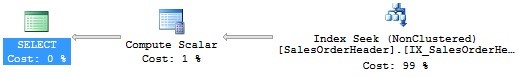
Table ‘SalesOrderHeader’. Scan count 1, logical reads 11, physical reads 0, read-ahead reads 0, lob logical reads 0, lob physical reads 0, lob read-ahead reads 0.

This query is run constantly, though, in order to locate the next order to package and ship. Despite the efficiency improvement, it still causes some contention and you’re asked to find an even faster alternative. A filtered index makes sense and you implement it as follows:

Once added, performance improves even more, with a subtree cost of 0.0045, an execution plan that looks identical to the previous one (though using the filtered index):

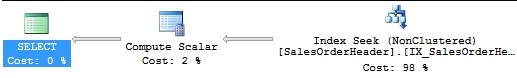
The STATISTICS IO shows a 9% reduction in reads:

Table ‘SalesOrderHeader’. Scan count 1, logical reads 10, physical reads 0, read-ahead reads 0, lob logical reads 0, lob physical reads 0, lob read-ahead reads 0.

Without some further design changes, our performance improvements stop here, but we have taken a problematic query and made it run very fast, even more so than the initial covering index allowed. The gains here may not seem huge, but if applied to a much larger table, can be invaluable. Let’s consider another example:

This query specifically looks for a small set of orders in which there is a specific offer and discount that is being applied. In order to cover this query, which is presumably run very often, we add the following index:

Once added, we can review the execution plan, STATISTICS IO, and also the STATISTICS TIME output:

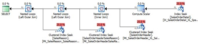
Table ‘SalesReason’. Scan count 0, logical reads 0, physical reads 0, read-ahead reads 0, lob logical reads 0, lob physical reads 0, lob read-ahead reads 0.
Table ‘SalesOrderHeaderSalesReason’. Scan count 41, logical reads 82, physical reads 0, read-ahead reads 0, lob logical reads 0, lob physical reads 0, lob read-ahead reads 0.
Table ‘SalesOrderHeader’. Scan count 0, logical reads 123, physical reads 0, read-ahead reads 0, lob logical reads 0, lob physical reads 0, lob read-ahead reads 0.
Table ‘Worktable’. Scan count 0, logical reads 0, physical reads 0, read-ahead reads 0, lob logical reads 0, lob physical reads 0, lob read-ahead reads 0.
Table ‘SalesOrderDetail’. Scan count 1, logical reads 4, physical reads 0, read-ahead reads 0, lob logical reads 0, lob physical reads 0, lob read-ahead reads 0.

SQL Server Execution Times:
    CPU time = 0 ms, elapsed time = 106 ms.

The subtree cost for this execution is 0.0132. Now, let’s add a filtered index to SalesOrderDetail in order to better cover this query:

After running this, the performance metrics now look like this:

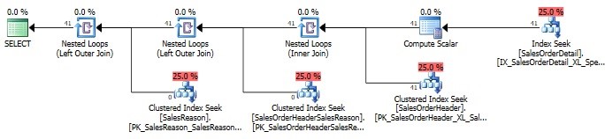
Table ‘SalesReason’. Scan count 0, logical reads 0, physical reads 0, read-ahead reads 0, lob logical reads 0, lob physical reads 0, lob read-ahead reads 0.
Table ‘SalesOrderHeaderSalesReason’. Scan count 41, logical reads 82, physical reads 0, read-ahead reads 0, lob logical reads 0, lob physical reads 0, lob read-ahead reads 0.
Table ‘SalesOrderHeader’. Scan count 0, logical reads 123, physical reads 0, read-ahead reads 0, lob logical reads 0, lob physical reads 0, lob read-ahead reads 0.
Table ‘Worktable’. Scan count 0, logical reads 0, physical reads 0, read-ahead reads 0, lob logical reads 0, lob physical reads 0, lob read-ahead reads 0.
Table ‘SalesOrderDetail’. Scan count 1, logical reads 2, physical reads 0, read-ahead reads 0, lob logical reads 0, lob physical reads 0, lob read-ahead reads 0.

SQL Server Execution Times:
    CPU time = 0 ms, elapsed time = 40 ms.

This time, the execution plan looks the same, and the reads are similar, though a bit lower. The runtime, though, is consistently less. In addition, the new index is smaller than the previous one. Here are the storage stats for the covering index with no filter applied:

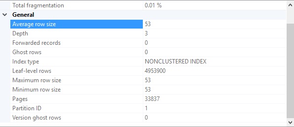
These are the storage stats for the filtered index:

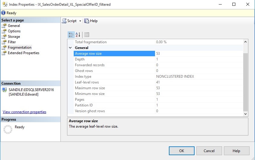
The unfiltered index takes up over 250MB of space, whereas the filtered index fits entirely on a single page! This not only saves valuable disk space, but reduces the time and resources consumed by index defragmentation processes.

We could build larger test tables to show more dramatic improvements, but there is more to tackle here than to show off what filtered indexes can do.

The Cost of Filtered Indexes

Whereas the benefits provided by all indexes are to improve read performance on specific columns or sets of columns for important queries, the cost paid for this is in write performance. With standard indexes, whenever a write operation is performed that happens to change columns included in an index, additional write operations need to be completed in order to update the index. As long as we properly maintain our indexes and don’t allow the number of them to get out of control, the read-write tradeoff we accept for those indexes is likely an excellent deal for us.

Filtered indexes contain additional metadata in the form of a WHERE clause, which can reference one or many columns, as illustrated in our previous examples. In addition to updating any sorting or include columns, the columns in the WHERE clause also participate in write operations when needed. This additional cost, when not accounted for, can result in unexpected latency or contention as SQL Server needs to check additional data values before updating the filtered index.

Let’s reconsider the second index we created above:

This index covers an important query by sorting on two columns, including three, and filtering on the same pair that were sorted on. A typical index update can be triggered with any write operation such as this:

This represents a fairly common update scenario, where we intend to update a single row based on the primary key values. The resulting execution plan shows the effort needed to accomplish this:

This shows the update of the clustered index, as well as the filtered index. The reads needed to complete this operation are relatively low:

Table ‘SalesOrderDetail’. Scan count 0, logical reads 3, physical reads 0, read-ahead reads 0, lob logical reads 0, lob physical reads 0, lob read-ahead reads 0.

Let’s try another example that will illustrate results that are not quite as expected. To begin, we’ll drop the filtered index created above:

With the index gone, we’ll run a simple query against an existing index on this table:

This is a simple update using an existing nonclustered index on ProductID in order to change the UnitPriceDiscount. The execution plan for it is, as above, the expected result:

The reads may seem high, but we are updating 9,348 rows in order to complete this statement:

Table ‘SalesOrderDetail‘. Scan count 1, logical reads 28673, physical reads 0, read-ahead reads 0, lob logical reads 0, lob physical reads 0, lob read-ahead reads 0.

Now let’s put the filtered index back into place:

When we run the same update statement from above, things get much more complicated:

An expensive key lookup has appeared in what was once an innocuous execution plan. IO on this operation, as expected, is also much higher:

Table ‘SalesOrderDetail’. Scan count 1, logical reads 56717, physical reads 0, read-ahead reads 0, lob logical reads 0, lob physical reads 0, lob read-ahead reads 0.
Table ‘Worktable’. Scan count 1, logical reads 18926, physical reads 0, read-ahead reads 0, lob logical reads 0, lob physical reads 0, lob read-ahead reads 0.

In addition to updating the clustered index on 9,348 rows, as we did above, we also performed an update on the filtered index as well. This additional update occurred, despite the fact that no rows in the result set matched the filter criteria for the filtered index. In other words, SQL Server had to verify the WHERE clause on the filtered index prior to determining if any updates had to be made, regardless of whether or not any rows were returned. This occurs because UnitPriceDiscount is in the include column list. A filtered index does not work in reverse: It is necessary to verify columns in the WHERE clause, even if no updates are required. The cost to perform this additional work was far from trivial, and if this query were run often, it could be crippling to a busy server.

Let’s run through a somewhat different example, this time on a query that does not update any columns that are included in the filtered index:

We are still targeting the index on ProductID with the WHERE clause, but are updating a different column that is not included in any indexes on Sales.SalesOrderDetail. Reviewing the execution plan and reads, though, reveals similar results to before:

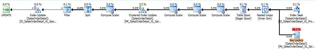
Table ‘SalesOrderDetail’. Scan count 1, logical reads 56717, physical reads 0, read-ahead reads 0, lob logical reads 0, lob physical reads 0, lob read-ahead reads 0.
Table ‘Worktable’. Scan count 1, logical reads 18884, physical reads 0, read-ahead reads 0, lob logical reads 0, lob physical reads 0, lob read-ahead reads 0.

In fact, everything looks exactly the same as it was before! Despite our not updating a column involved in the index at all, SQL Server still went through the trouble of checking the WHERE clause anyway. If we remove the index, the execution plan and IO return to what we would expect of this query:

Table ‘SalesOrderDetail’. Scan count 1, logical reads 28673, physical reads 0, read-ahead reads 0, lob logical reads 0, lob physical reads 0, lob read-ahead reads 0.

Conclusion

The effects of adding a filtered index were far more significant than would be expected for some of the queries presented above. It may be easy for a DBA to forget that a filtered index would influence any other queries that update data within it. The fact that unrelated queries still caused unnecessary reads in order to essentially complete a no-op is not something anyone would assume.

Based on these experiences, I am now much more cautious towards filtered indexes. In any scenario where I would consider them, I would feel obliged to do research into common write operations on the table to ensure they won’t be adversely affected by the new index. Regardless of whether the write operations affect columns within a filtered index, we would want to be vigilant anyway to ensure that we are not being harmed either by carelessness or unexpected behavior.

Microsoft has a Connect article that addresses this bug, submitted by Paul White.

It is unclear if this issue will be addressed in the future. My hope is that Microsoft will take a feature that appeared to be a cure-all for queries on large tables and improve it so that we aren’t sideswiped by unexpected performance problems.

• Author
• Recent Posts

Ed Pollack

Ed has 20 years of experience in database and systems administration, developing a passion for performance optimization, database design, and making things go faster.He has spoken at many SQL Saturdays, 24 Hours of PASS, and PASS Summit.This lead him to organize SQL Saturday Albany, which has become an annual event for New York’s Capital Region.

In his free time, Ed enjoys video games, sci-fi & fantasy, traveling, and being as big of a geek as his friends will tolerate.

View all posts by Ed Pollack

Latest posts by Ed Pollack (see all)

• SQL Server Database Metrics - October 2, 2019
• Using SQL Server Database Metrics to Predict Application Problems - September 27, 2019
• SQL Injection: Detection and prevention - August 30, 2019