
Introduction
One of a database designers’ worst nightmares is having to design a database for business analysts and data stewards whom insist upon creating their own reports, using Excel as a GUI. The reason that I mention this is that user created reports often open up “Pandora’s box”; with many of these folks creating their own ‘miss-information’ due to a lack of understanding of the underlying data. A few weeks back I had the ’fortune’ of working on such a project, which prompted an ‘ah-ha’ moment. I decided to design the backend SQL Server database using the Business Intelligence Semantic Model (BISM) and to employ the super set of tools provided by Microsoft Power BI, with Excel as a GUI. The end results were wildly accepted by the user community and once you see how easy this is to apply, you will be ‘chomping on the bit’ to employ the same techniques on your own user driven projects.
The preliminary research
Upon examining the existing data stores, I noted that most of the client’s data resided in spreadsheets. In order to show you the reader how we accomplished the conversion, I shall be using non confidential data readily available on the internet.
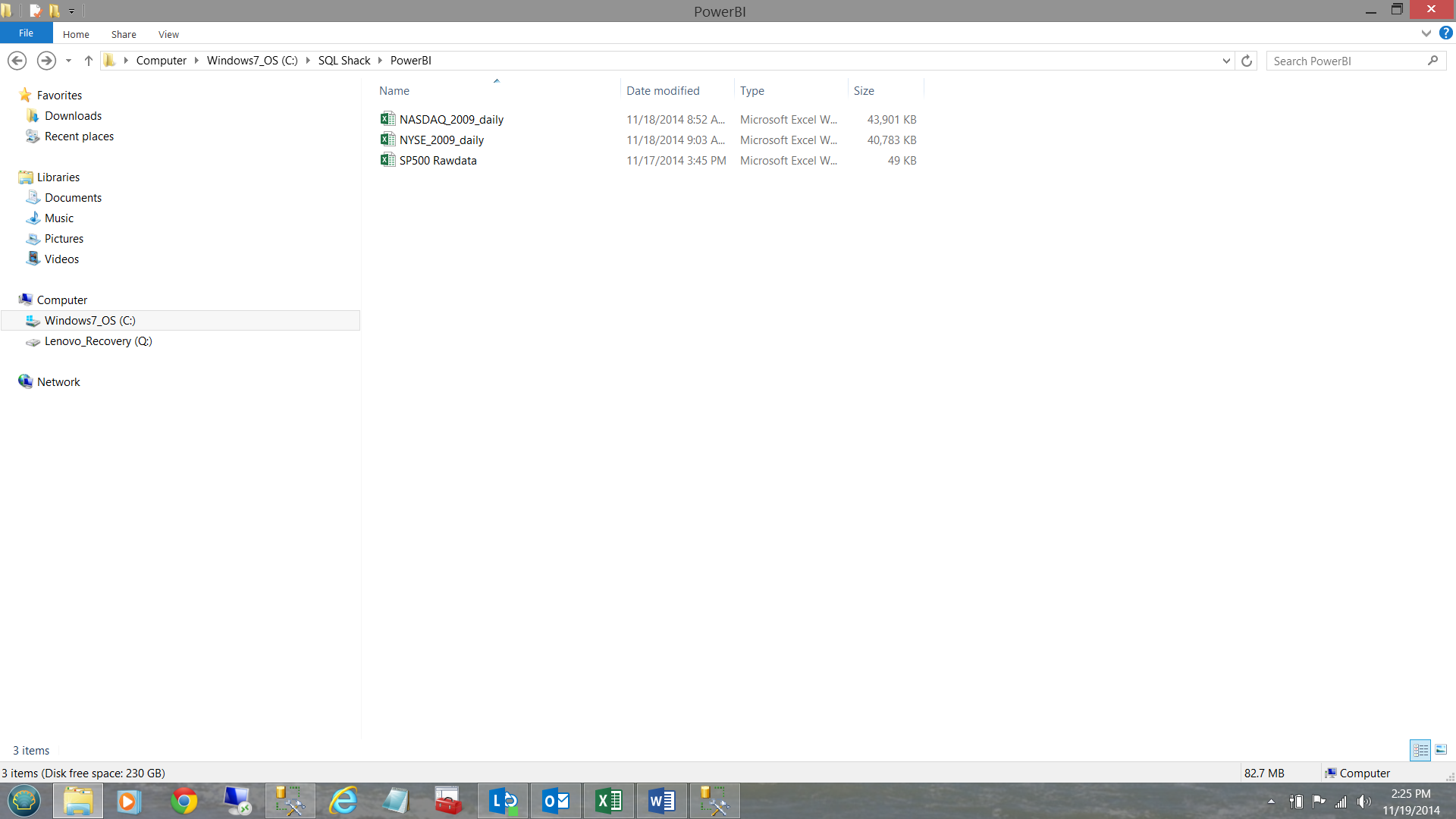
Our first step is to load the data from these spreadsheets into a relational database which I have called ‘SQLShackFinancial’. The spreadsheets contain data from varied exchanges such S&P, NYSE and the NASDAQ.
As a final note, this exercise utilizes SQL Server 2012 Enterprise Edition or SQL Server 2012 Developer Edition as this is the first version that offers Tabular Model facilities. You may also utilize the same 2014 editions.
Getting started
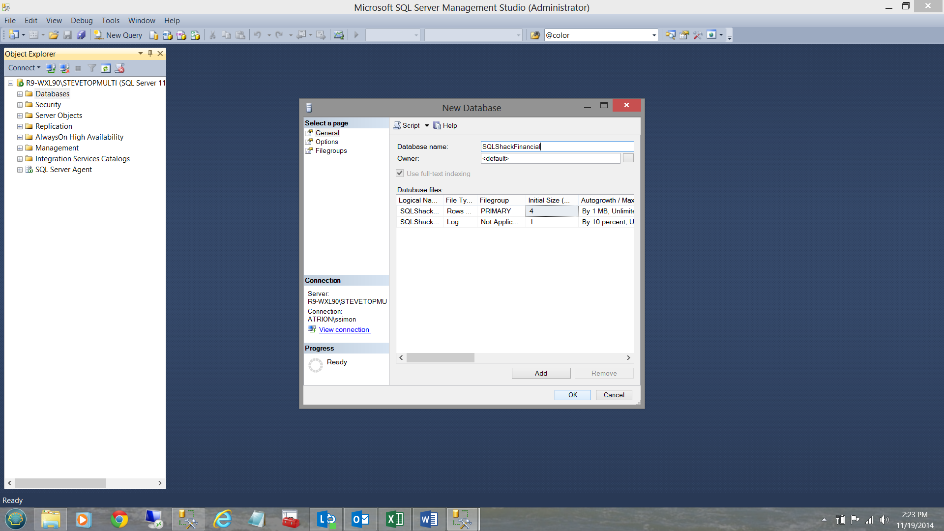
We begin our journey within SQL Server Management Studio (SSMS) by creating a normal relational database called ‘SQLShackFinancial’ (see below).
Our next task is to load the data from the spreadsheets shown below:
Now, we could use the ‘load wizard’ within SSMS, however the wizard is great for one offs. In our case the client wishes to reload the tables on a daily basis and therefore we shall opt for creating an SQL Server Integration Services package.
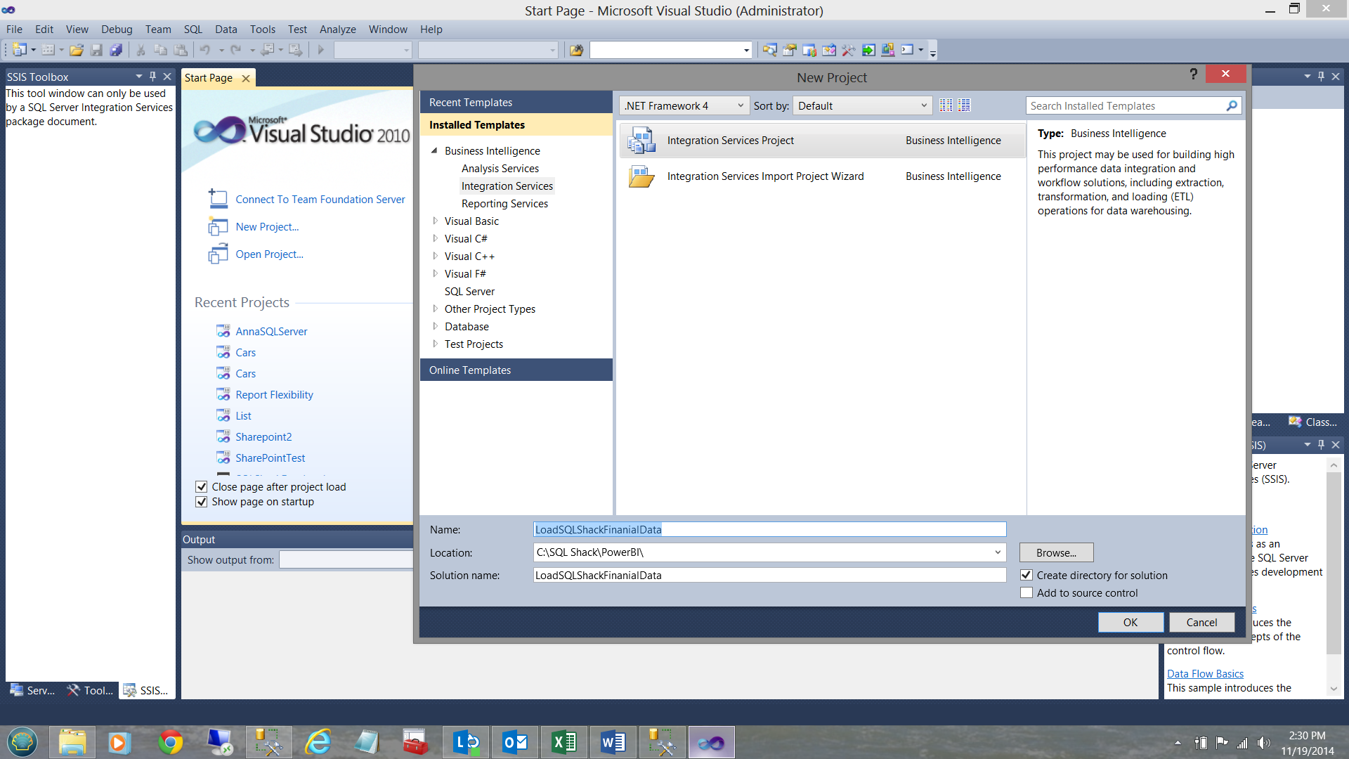
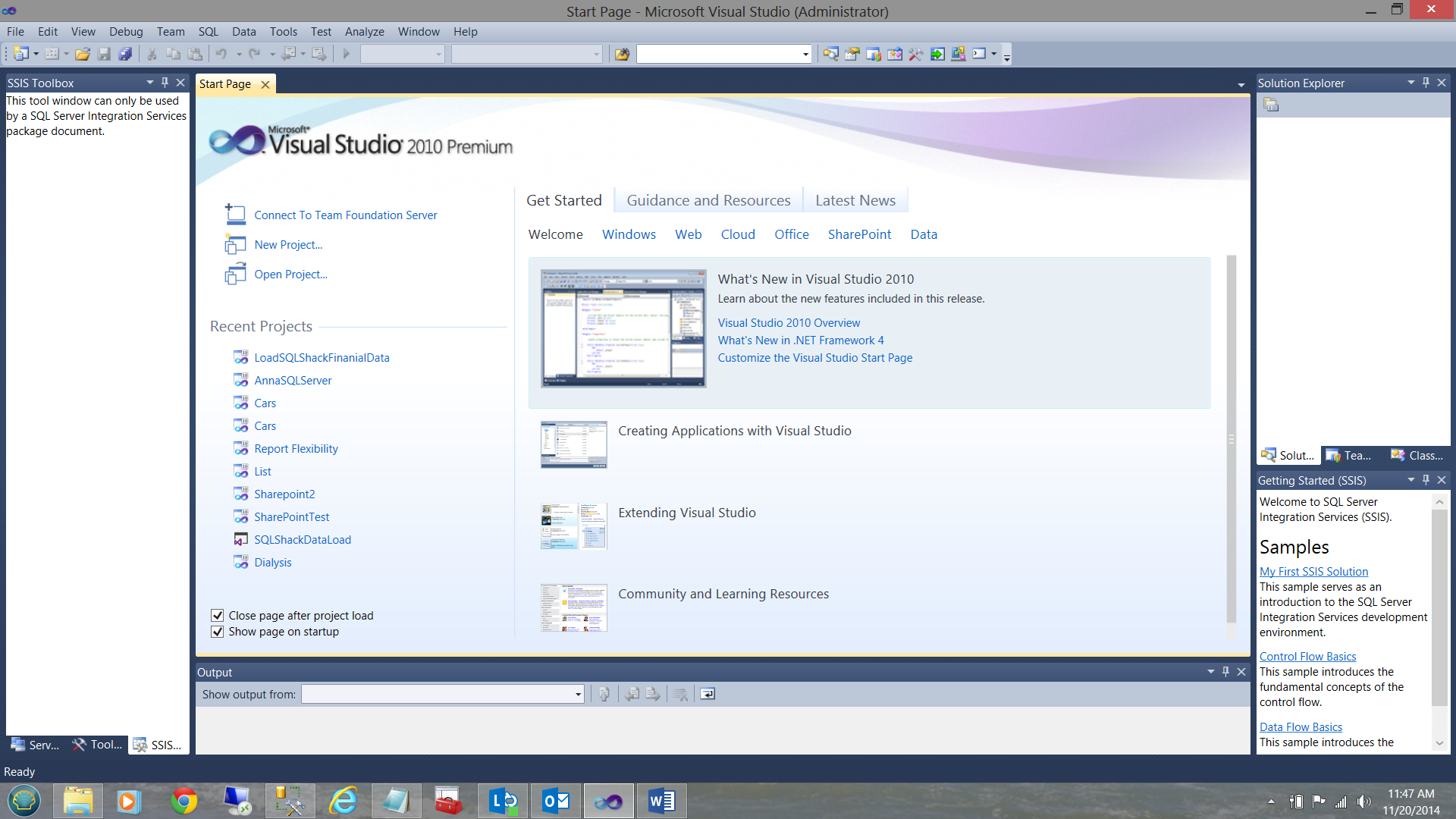
I start by bring up SQL Server Data Tools (SSDT) and creating a new SQL Server Integration Services package. I call my project ‘LoadSQLShackFinancialData’ (see below).
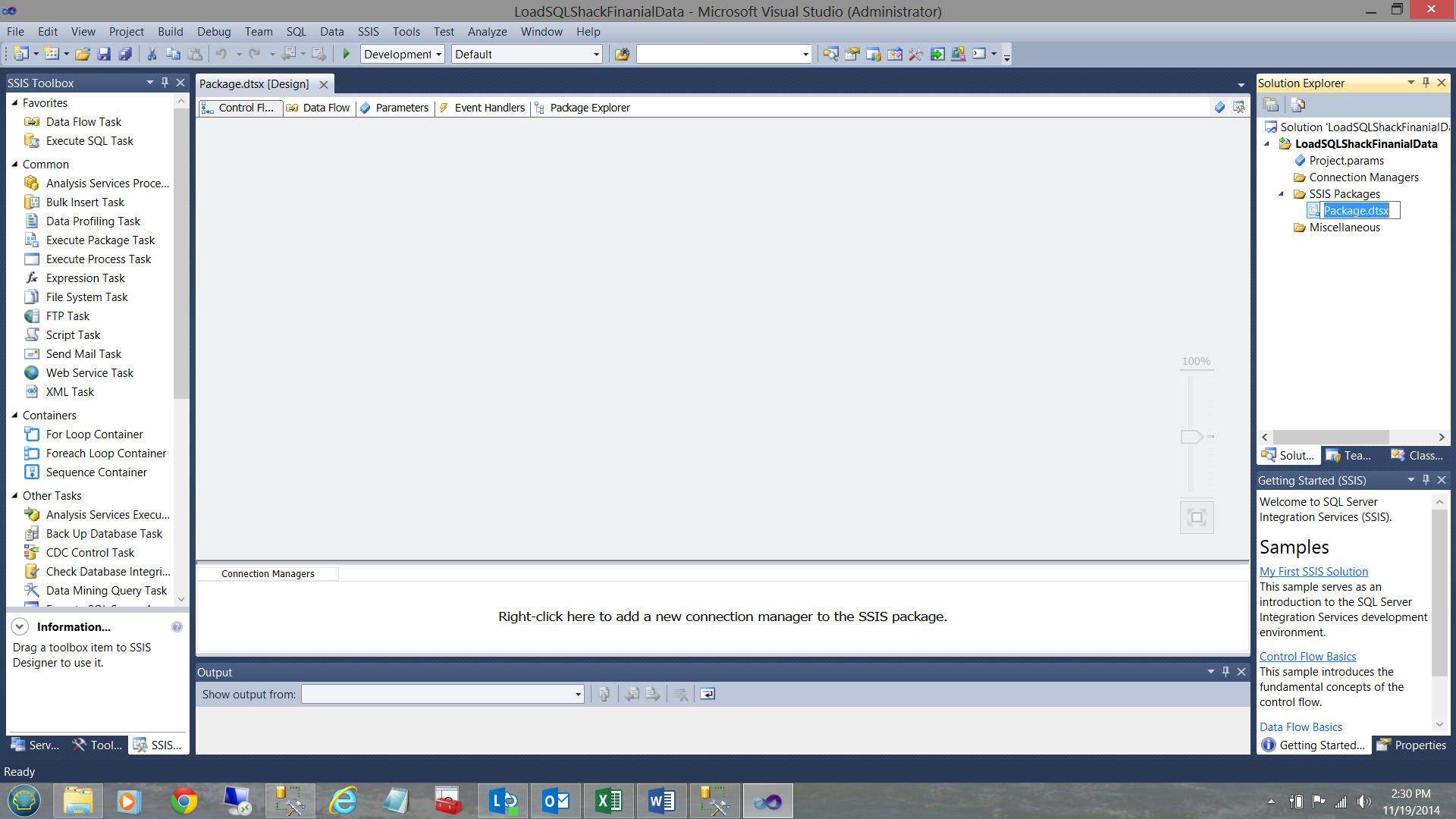
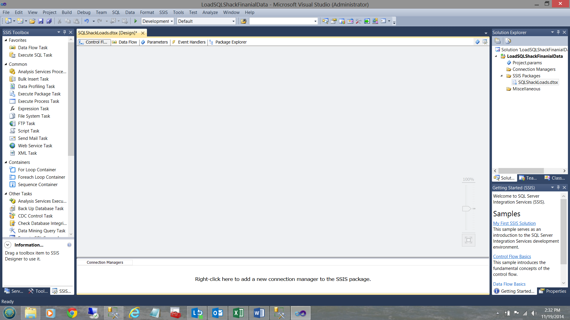
Upon clicking OK to create the package, I arrive at ‘Control Flow’ work surface where I shall begin to structure the load package.
I rename the package to ‘SQLShackLoads’.
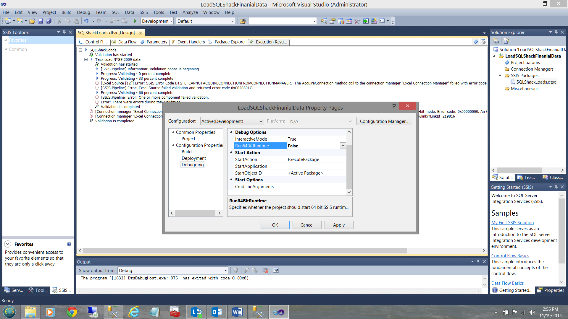
Clicking on the project tab of the menu bar, I call up the project properties page. I expand the ‘Configuration Properties’ menu and set the Run64BitRunTime to ‘False’ (see above). I click apply and OK.
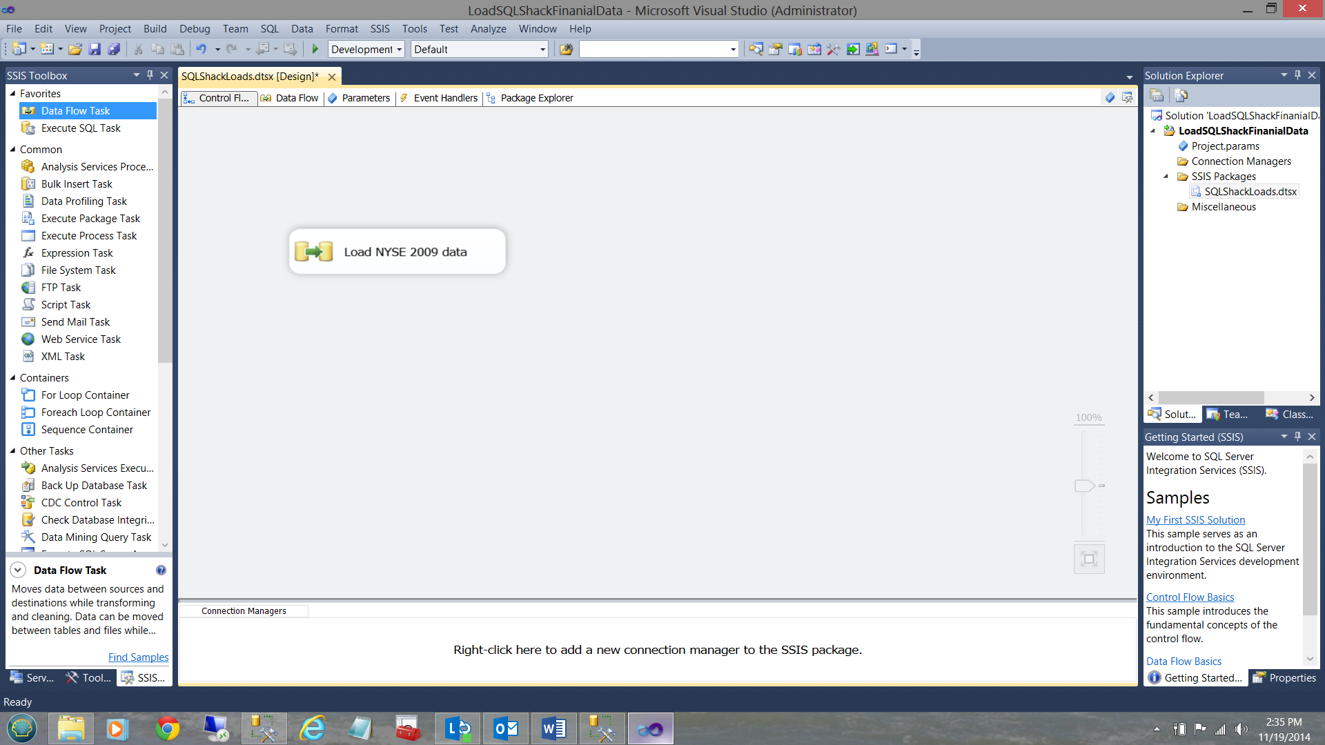
I now drag a ‘Data Flow Task’ onto the working surface of the Control Flow and rename that Data Flow ‘Load NYSE 2009 data’ (see below).
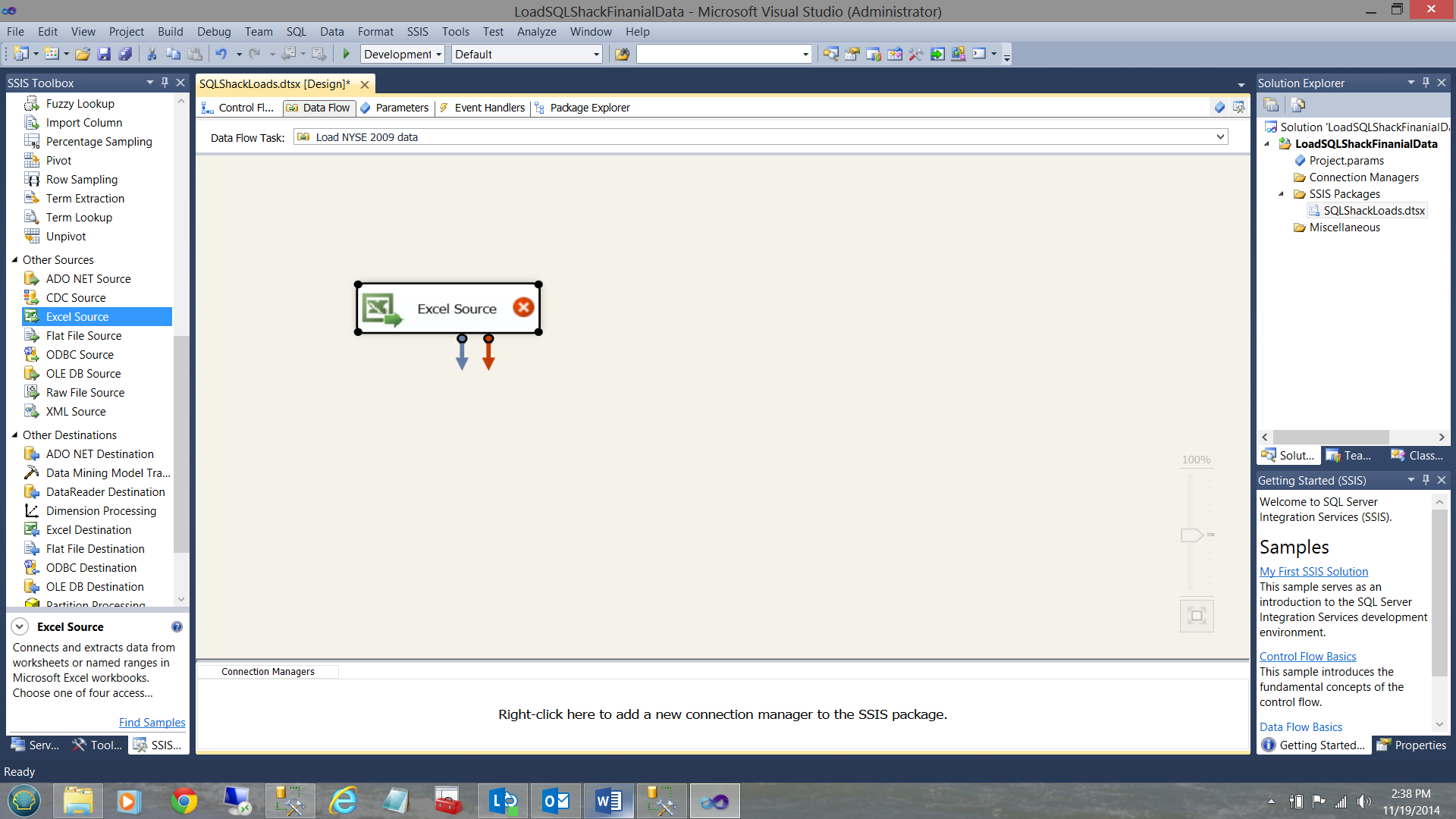
Double clicking on the data flow (see above) we are brought to the ‘Data Flow’ tab. I add an ‘Excel Data Source’ (see below)
I merely configure this data source to point to my NYSE Excel Workbook.
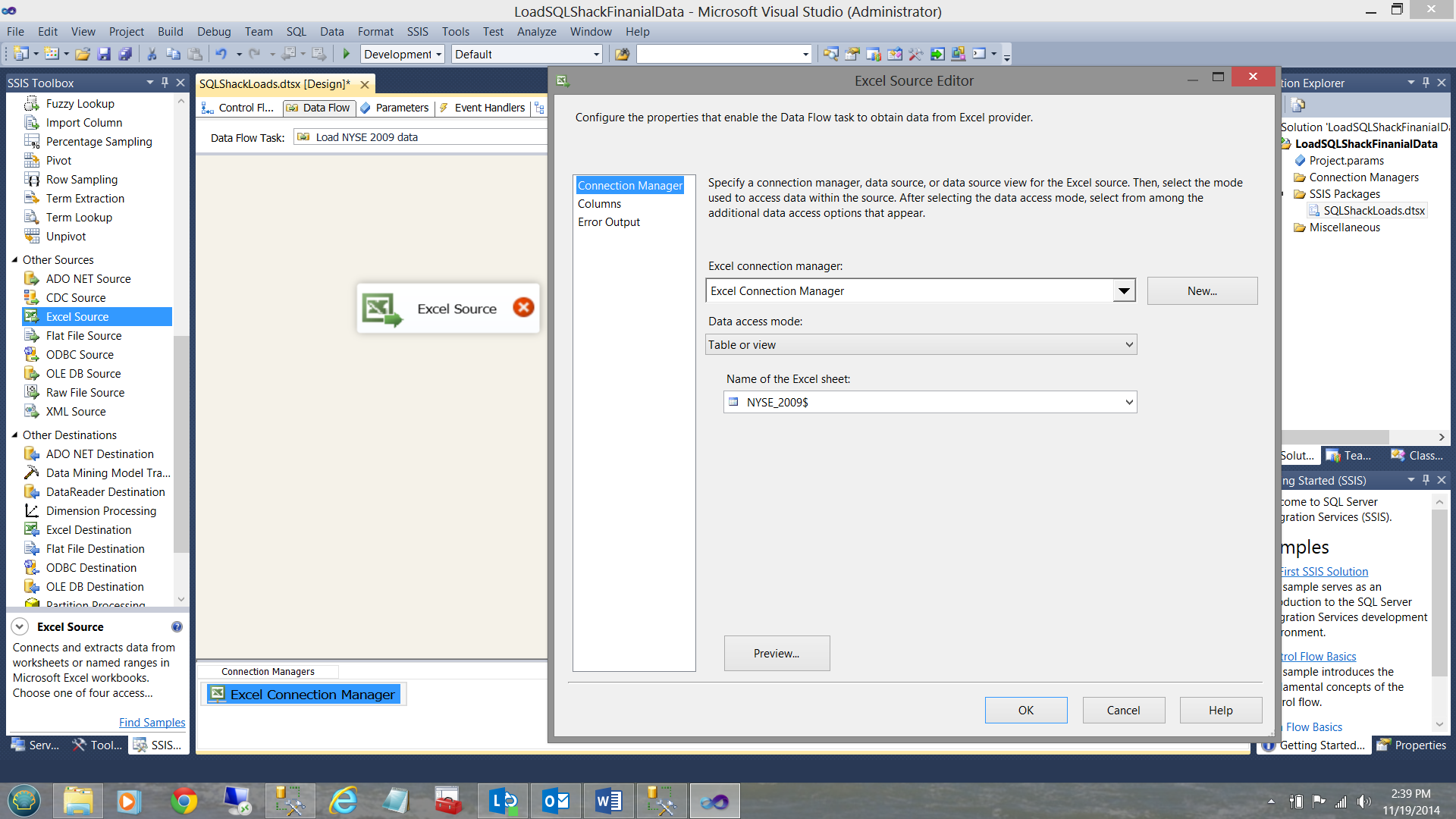
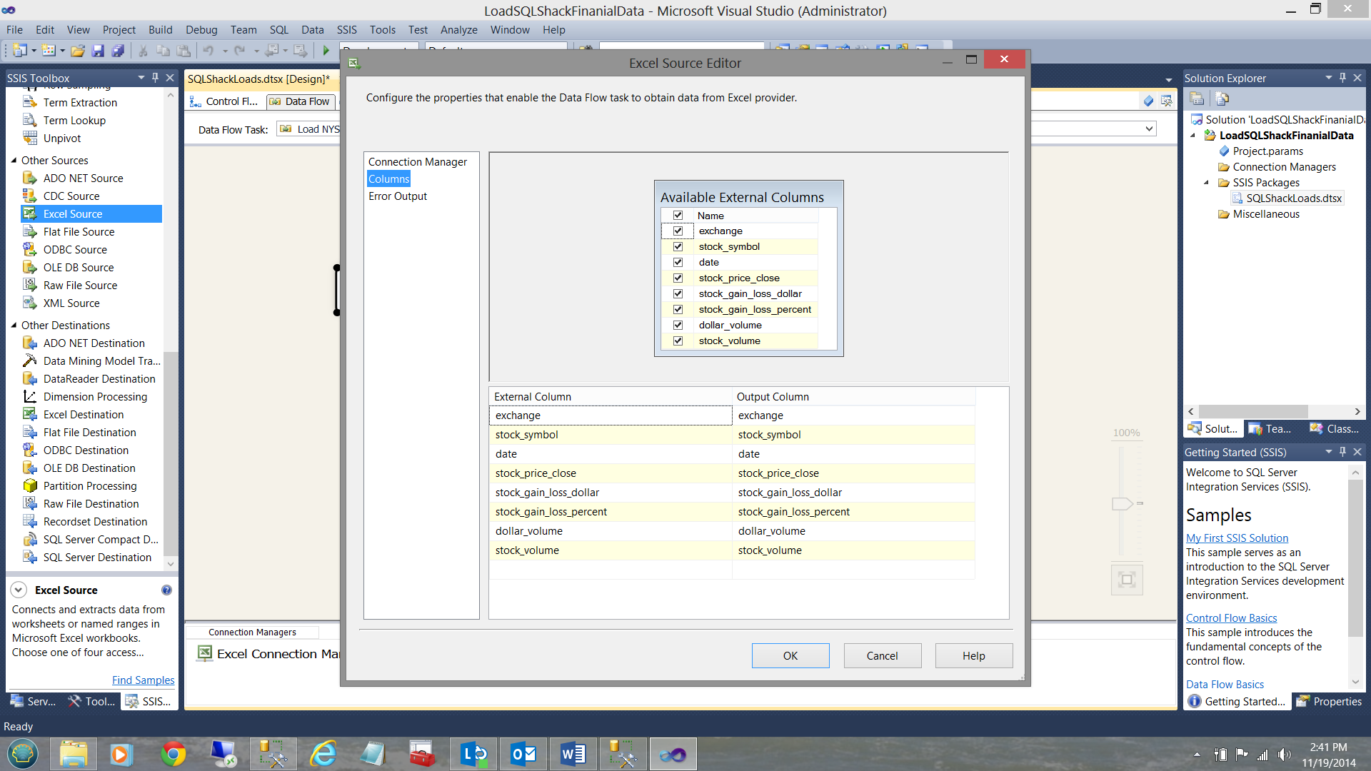
And view my incoming data columns (see below).
I now click OK to leave the ‘Excel Source’ configuration screen, having defined my data source.
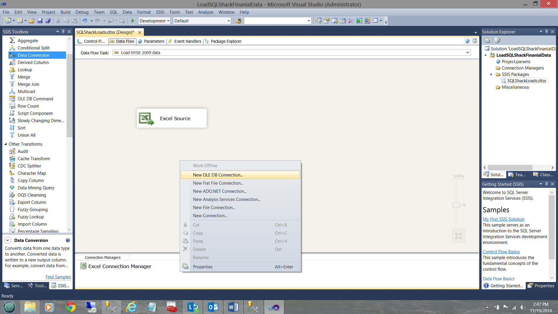
Our next step is to create a data connection to our SQL Server database so that the data from the Excel data source may be placed in a table within the database. I right click within the Connection Managers box and create a new OLE DB connection (see below).
We must now configure this connection (see below).
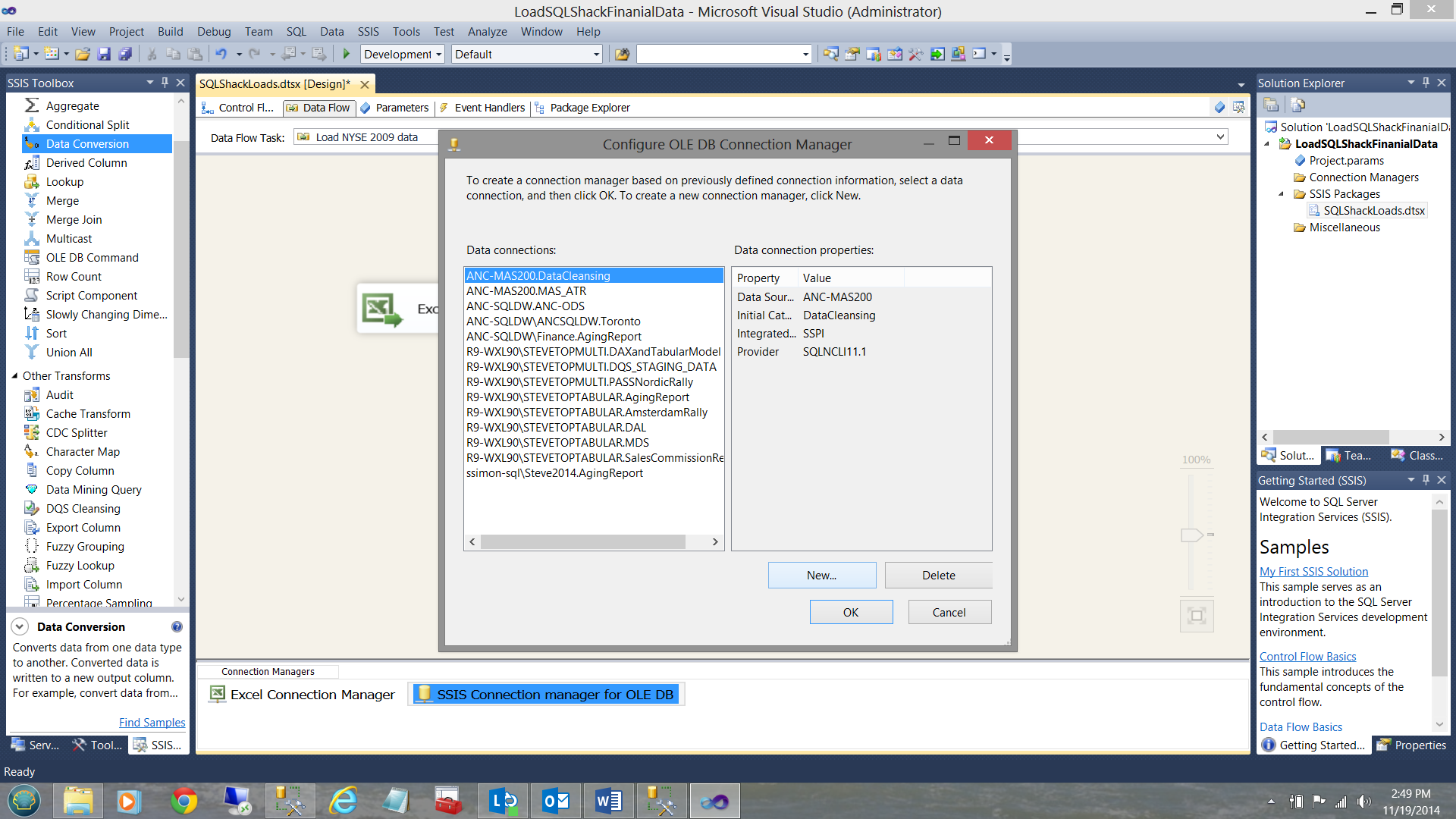
As this is the first time attempting to access the SQLShackFinancial database, we create a ‘new connection’. I click on the ‘New’ button shown above. The connection manager data collection screen is brought into view.
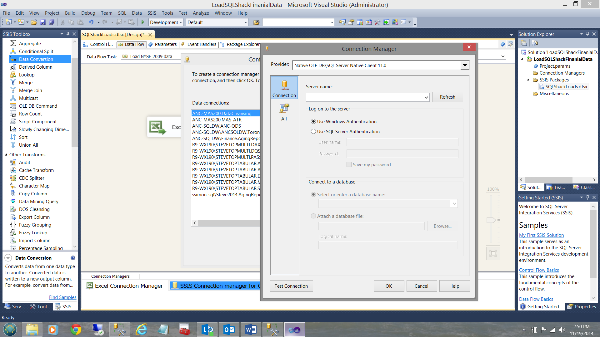
I merely complete the ‘Server name’ box, tell SSIS which database I wish to connect to, and test the connection. The completed data entry screen is shown below.
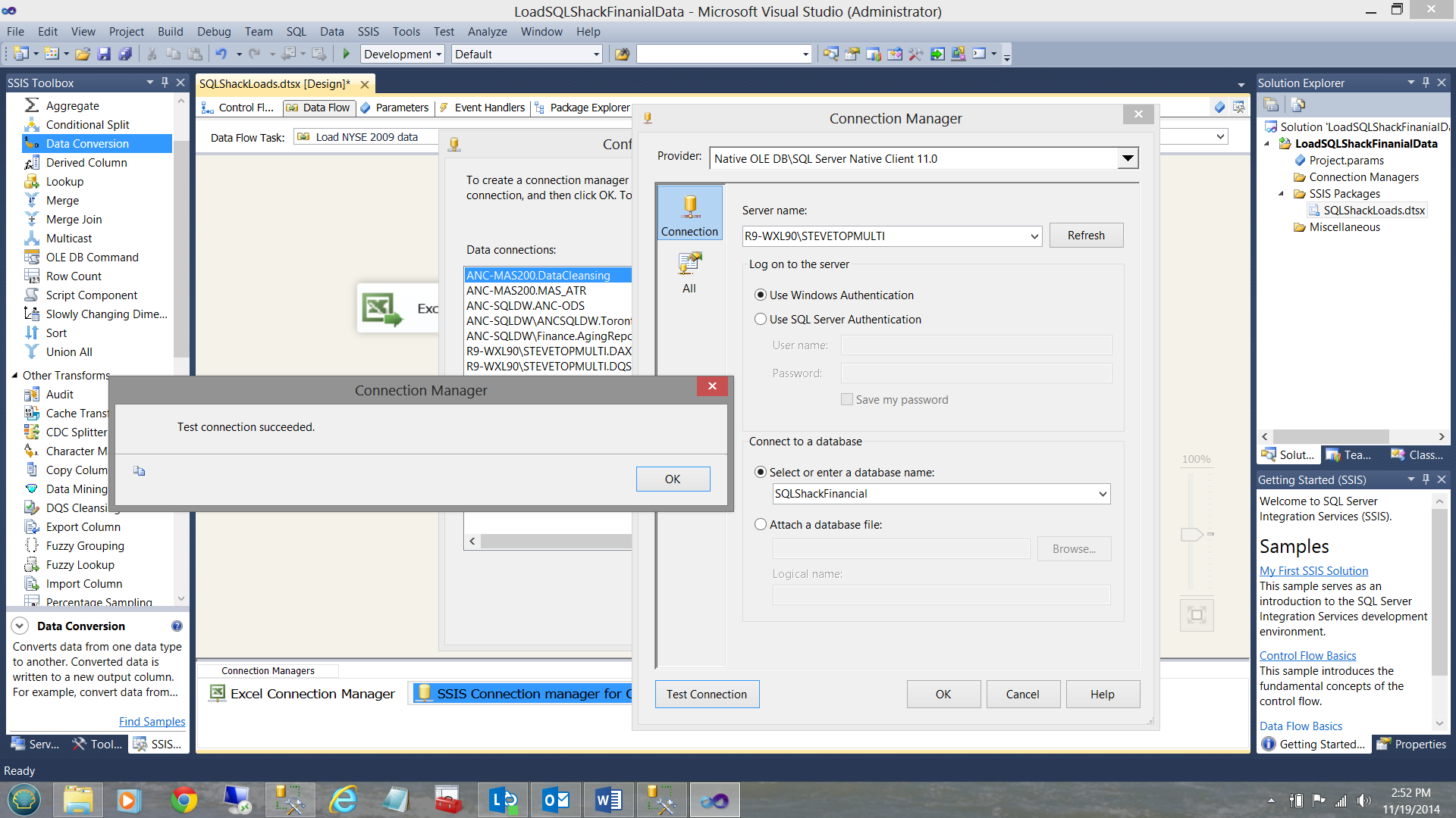
Finally, I click OK, OK and OK again to return to my ‘Data Flow’ screen.
We do have one issue with this data: the date field within the spreadsheet is a ‘text’ field (see below).
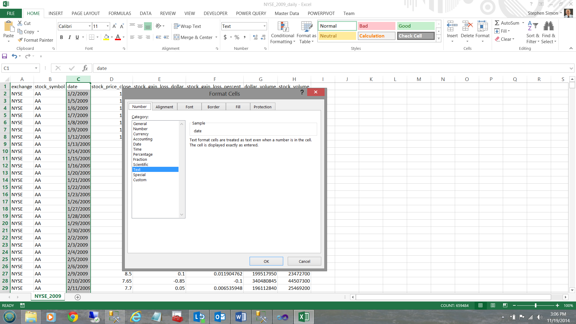
This is not really optimal as I know that I shall be doing date related queries. Therefore upon loading the data into our database table I shall convert it to a date, prior to actually inserting it into the table. To achieve this, I add a ‘data conversion’ control onto the design surface (see below).
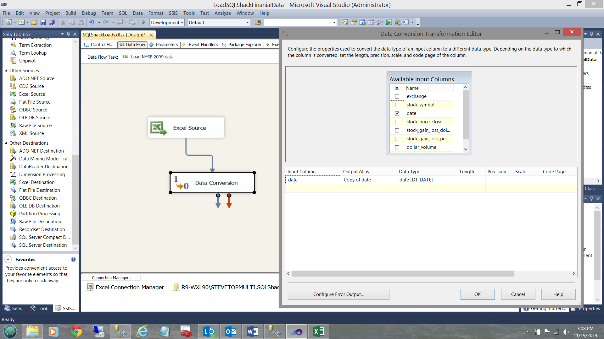
Opening the control, I check the ‘date’ input column and change the data type of the output to ‘DT_DATE’ and click OK. Our final step in the process is to add an OLE DB destination control which will connect the data flow to our final data repository table (see below).
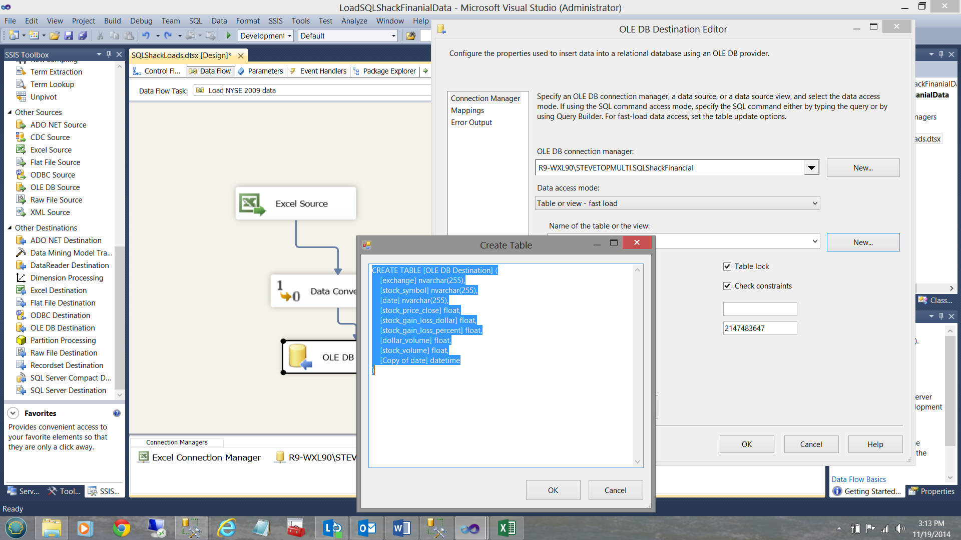
By double clicking the ‘OLE DB Destination’ that we just brought onto our surface, the OLE DB Destination Editor is brought up. I point it to the SQLShackFinancial connection that I created above and I click the ‘New’ button for the ‘Name of the table or the view’ option. We must remember that the table does not yet exist as this is the first time that I am loading data into the database.
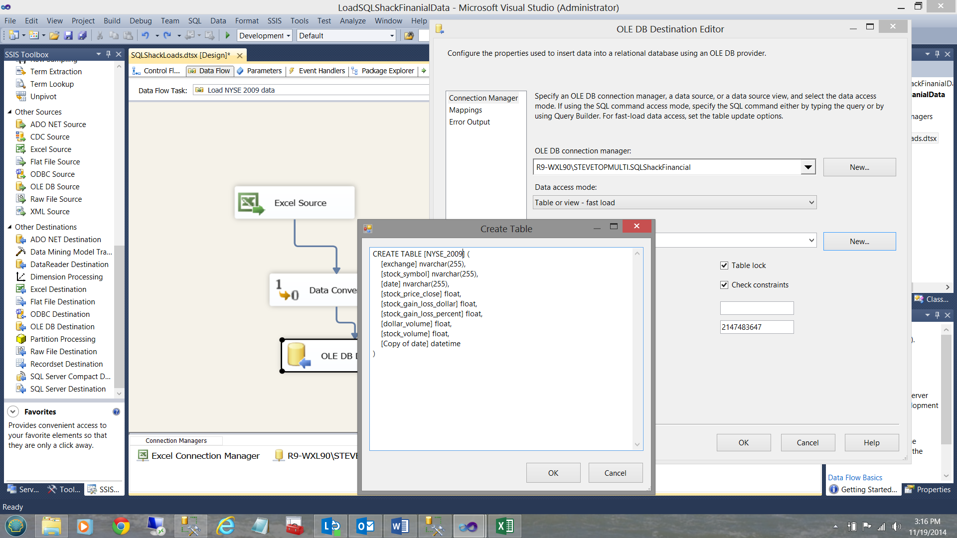
I name the table NYSE_2009 and click OK (see below).
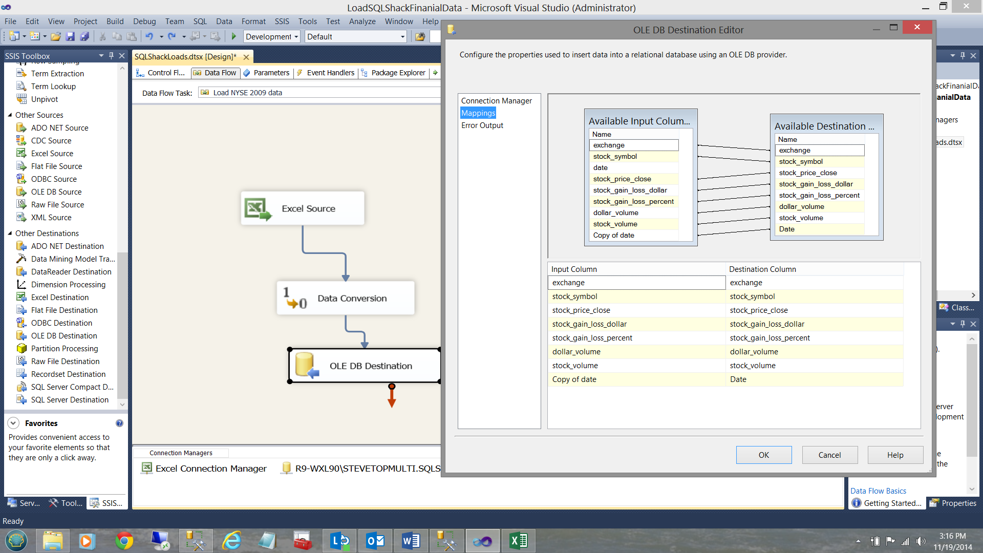
Clicking the ‘Mappings Table’, I am now able to link the incoming fields with the final fields within the database.
We are now in a position to load the table.
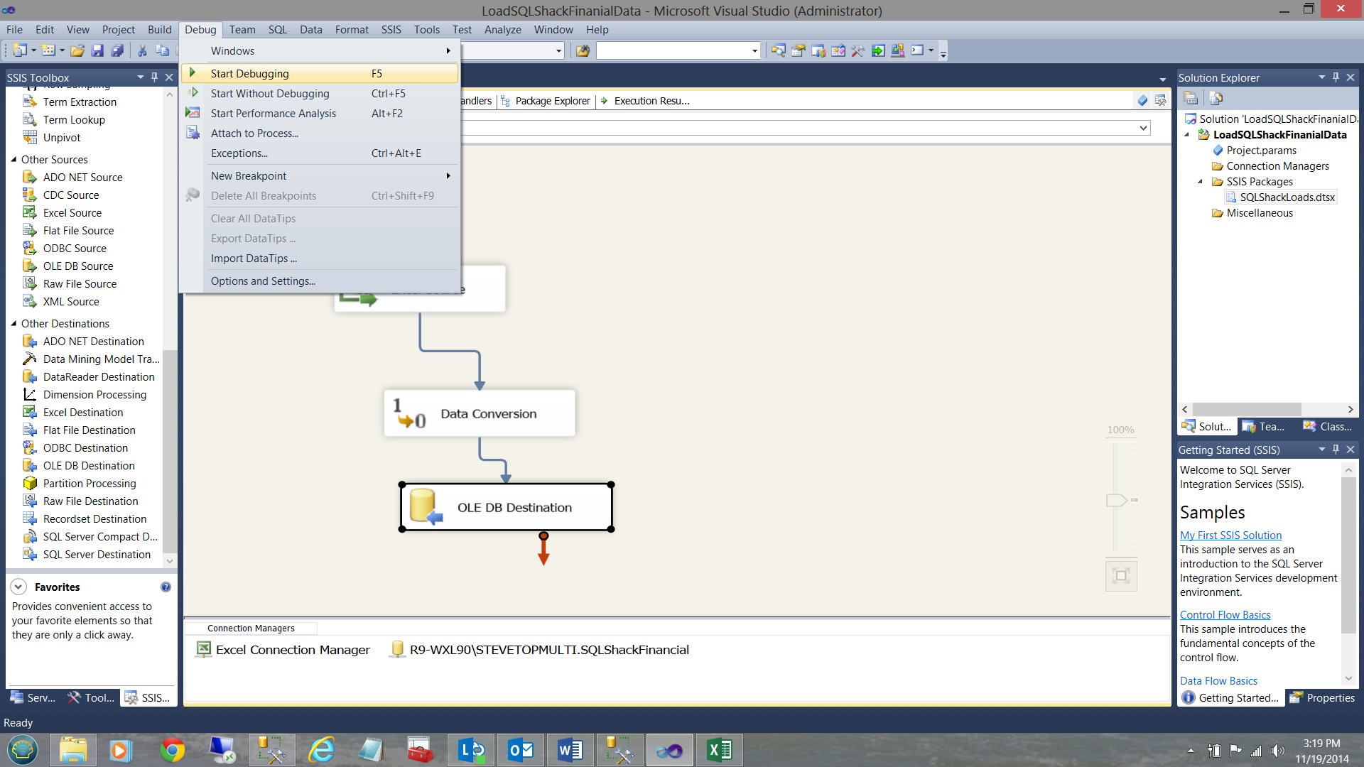
As a one off, I shall execute the load manually (as setting up the load to run as a batch job is outside the scope of this paper). I click on the ‘Debug’ table and select ‘Start Debugging’ (see above).
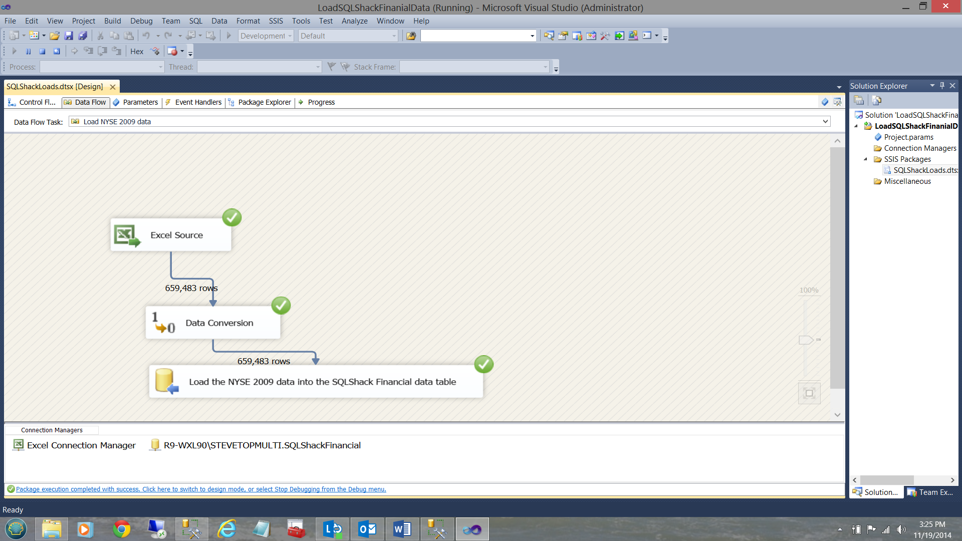
When the load is complete, the screen will appear as shown below:
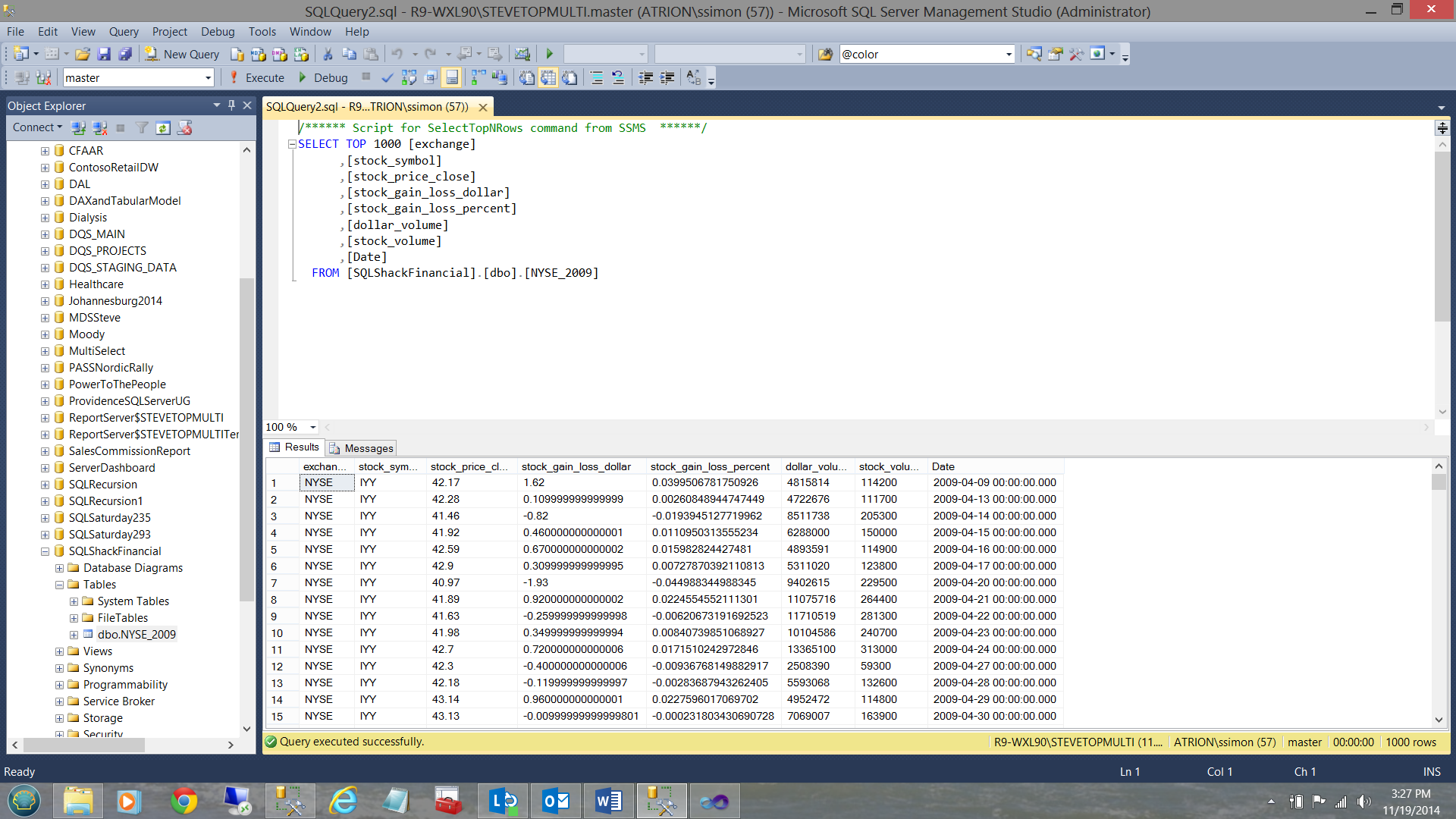
Meanwhile, back in SQL Server Management Studio, the data that we just loaded may be seen below:
It is left up to the reader to repeat the same steps to load the NASDAQ and S&P data in a similar manner to that shown above.
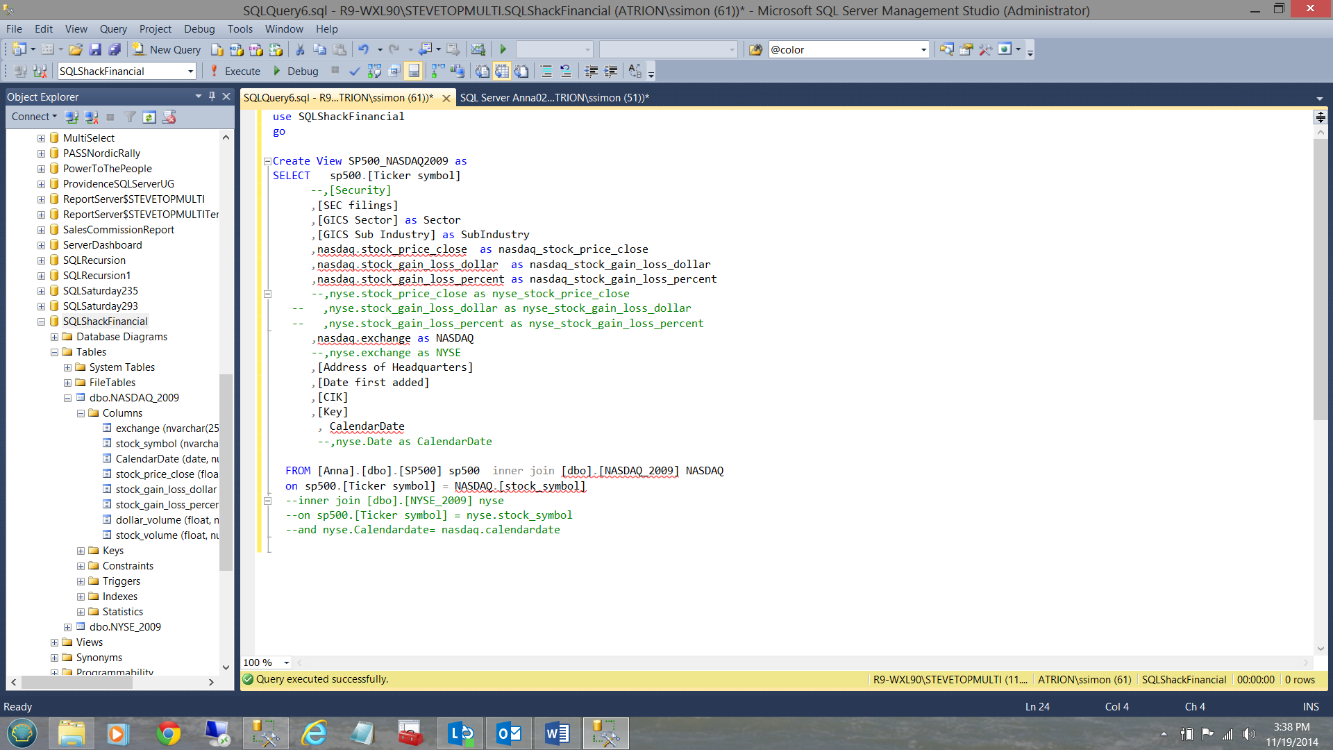
We shall now create two views, one of which will be used to link the S&P 500 table to the NYSE_2009
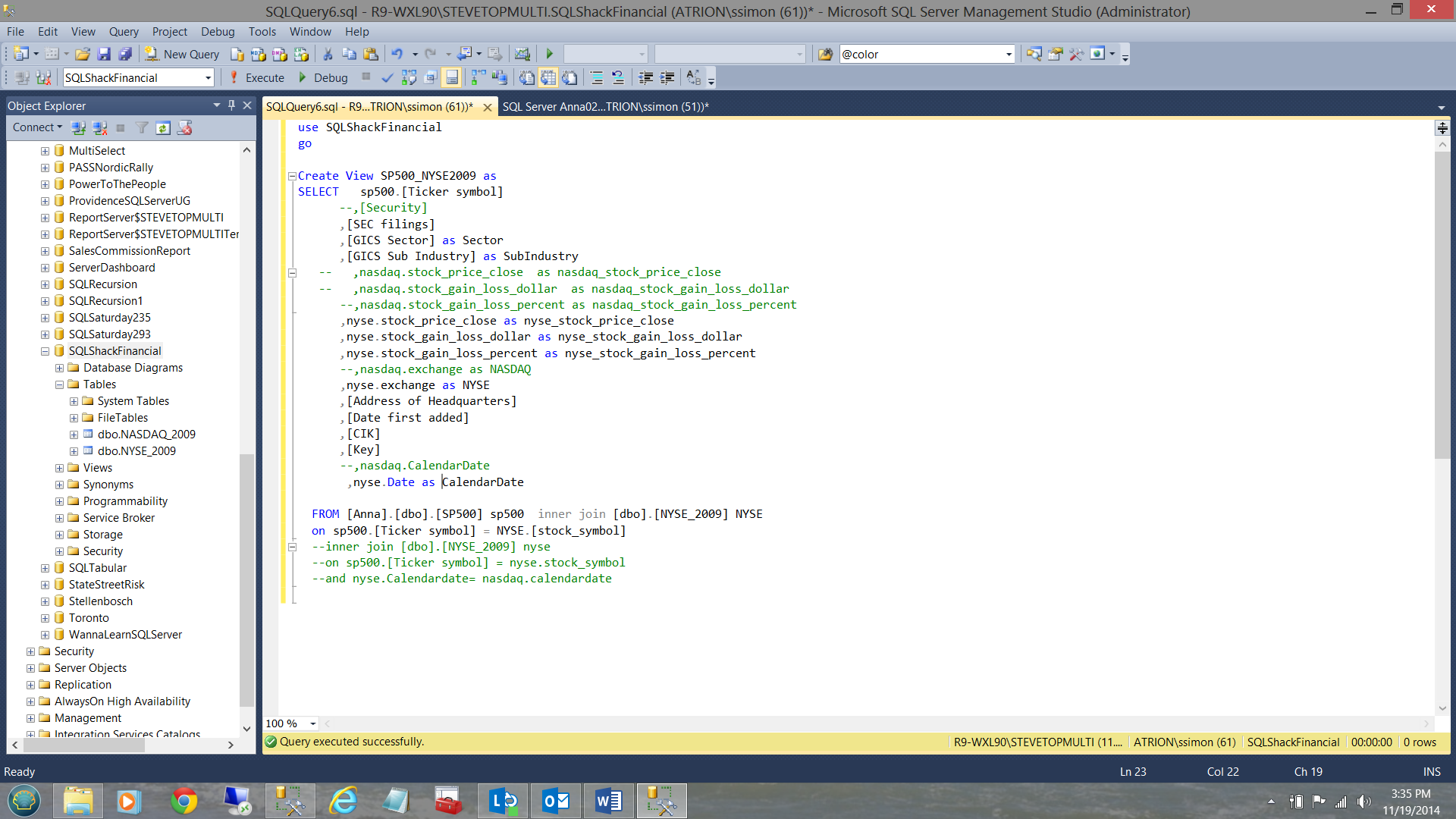
and the other to link the S&P 500 table to the NASDAQ_2009 table (see below).
Constructing our Tabular Analytic Solution
After much thought and design, I chose to utilize the tabular model. Not only does the tabular model give users the look and feel of a spreadsheet, it also permits us to create our own microcosm which is not easily established utilizing conventional multi-dimensional modeling.
To begin we bring up SQL Server Data Tools (SSDT) and this time we are going to create and ‘Analysis Services Tabular Project’.
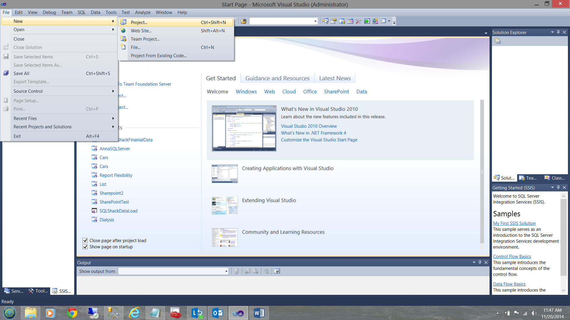
We click ‘New’ and select ‘Project’ from the main menu (see above). A further menu is then displayed. We select ‘Analysis Services Tabular Project from the ‘New Project’ menu (see below).
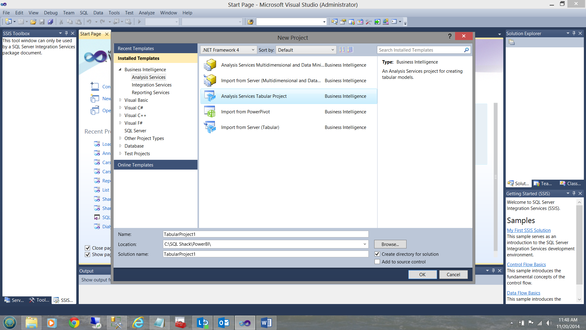
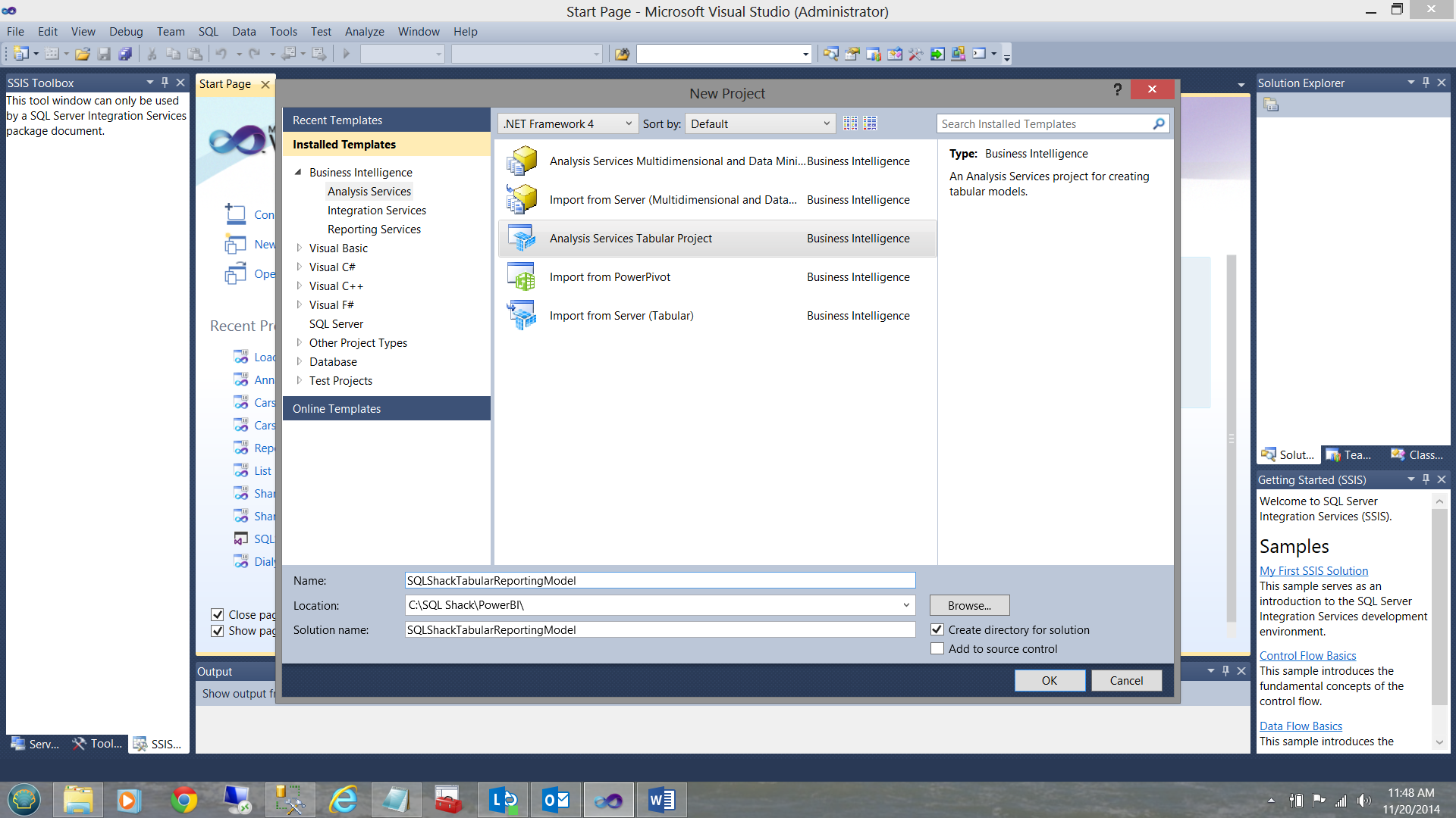
I give the project a name. In our case I call it ‘SQLShackTabulaReportingModel’, and click OK (see below).
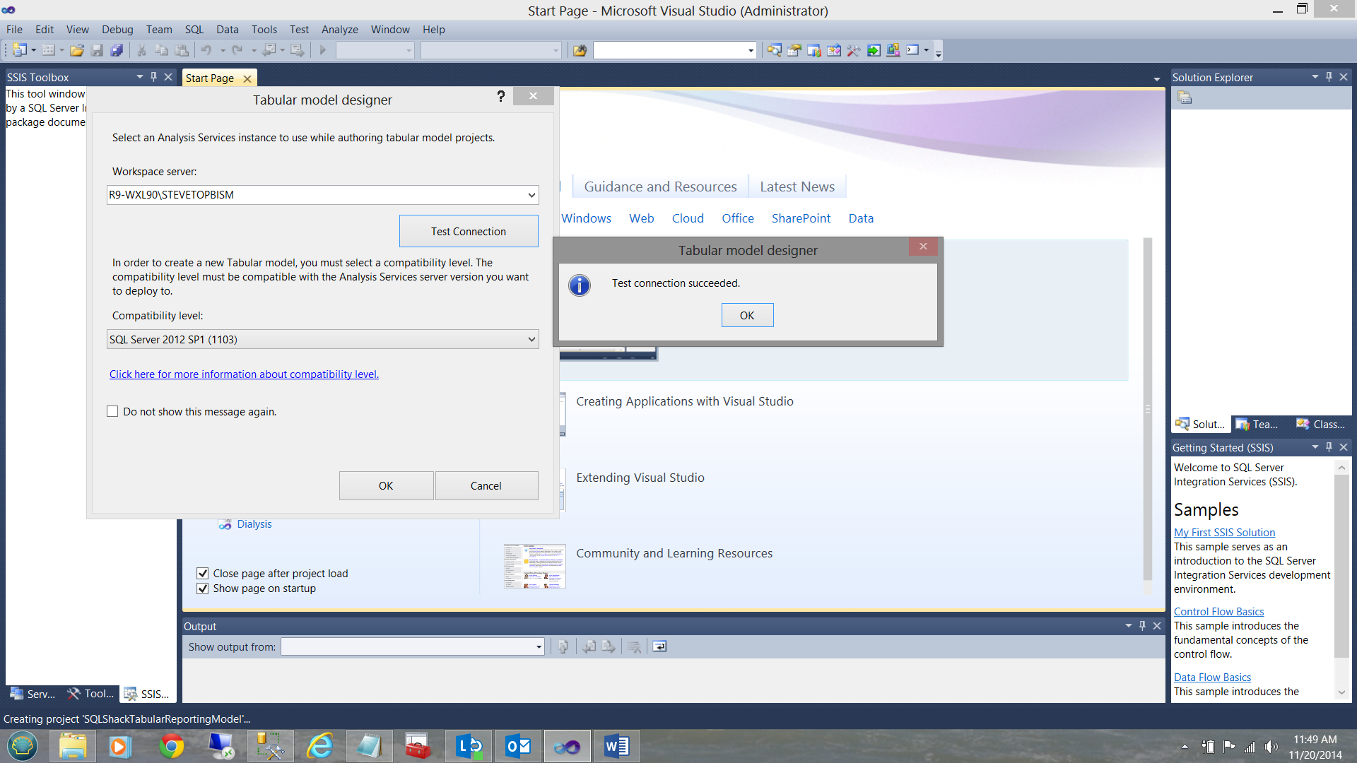
The system now asks me where the end project will reside, i.e. on which Analysis Services server. Having created the connection, I test it and I am informed that all is in order (see below).
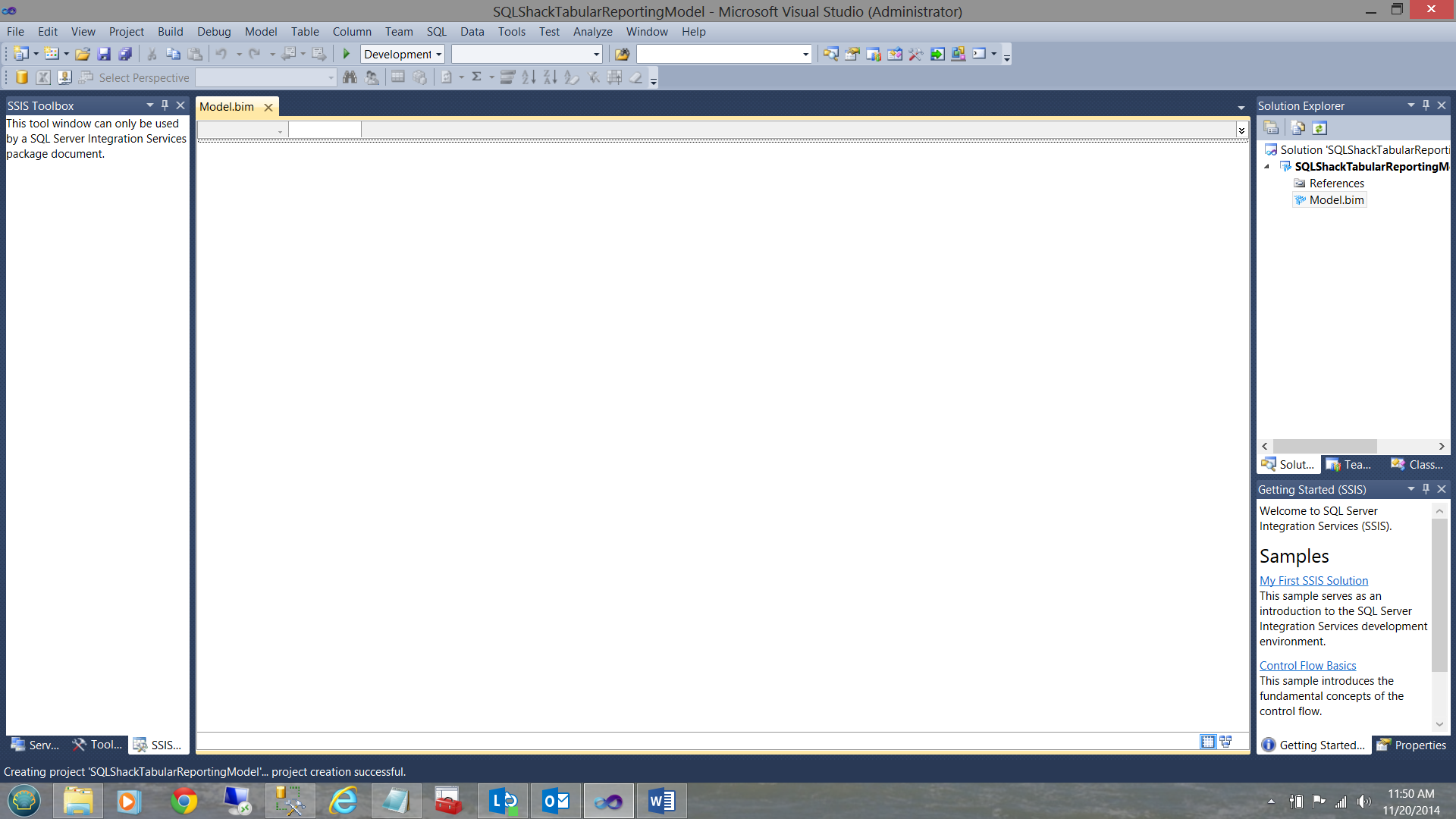
Having configured our project, we now arrived at our main work surface (the data model). Whilst we have defined where our end project will reside, we have yet to define the data source.
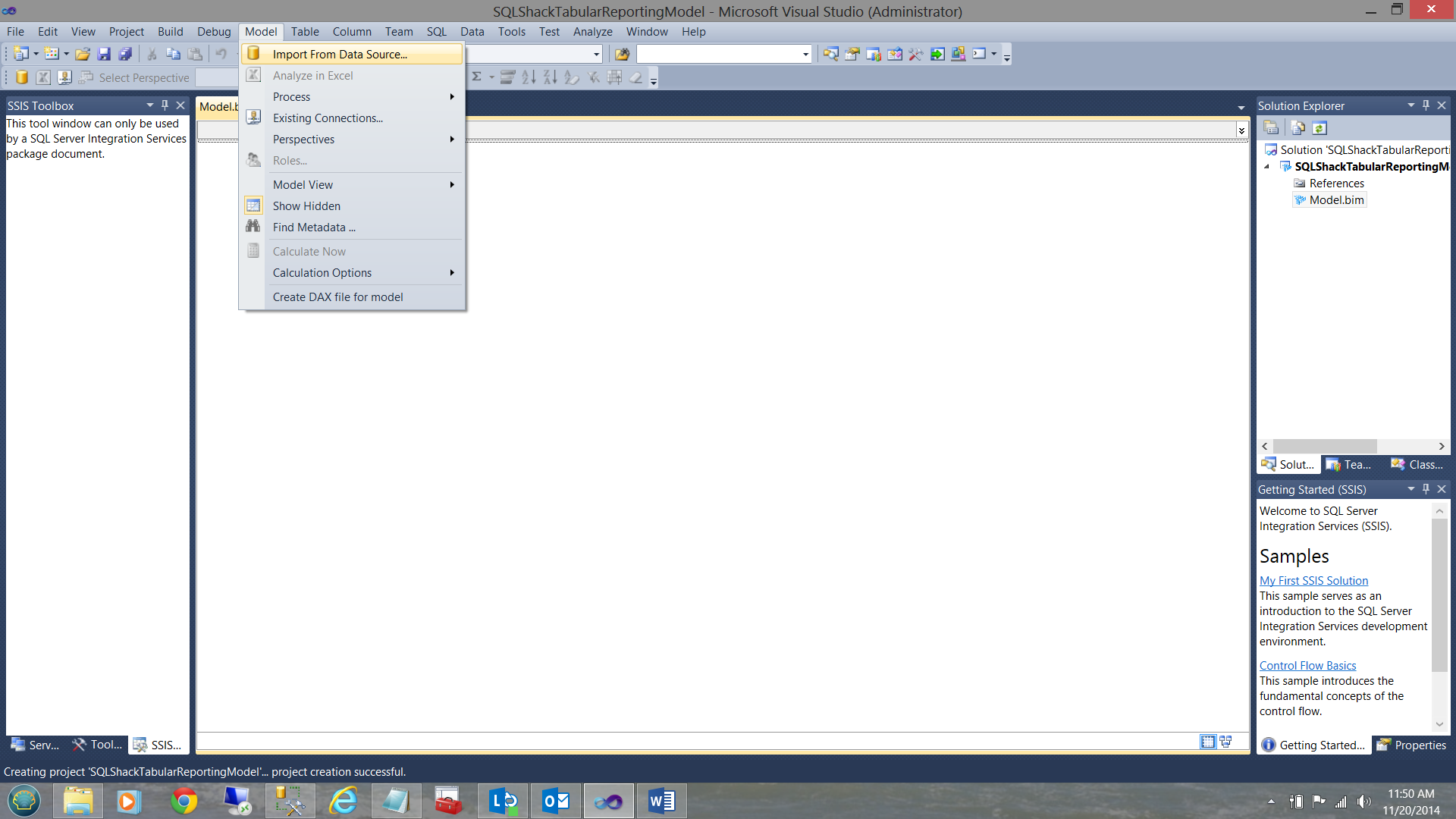
I click ‘Model’ and then “Import from Data Source’.
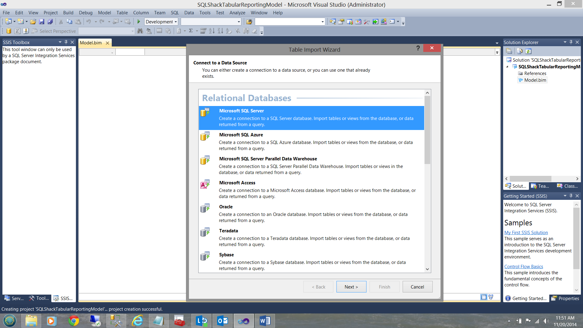
The ‘Table Import Wizard’ is brought up. I choose a ‘Microsoft SQL Server’ data source (see above). The ‘Define your data source’ input screen is now displayed (see below).
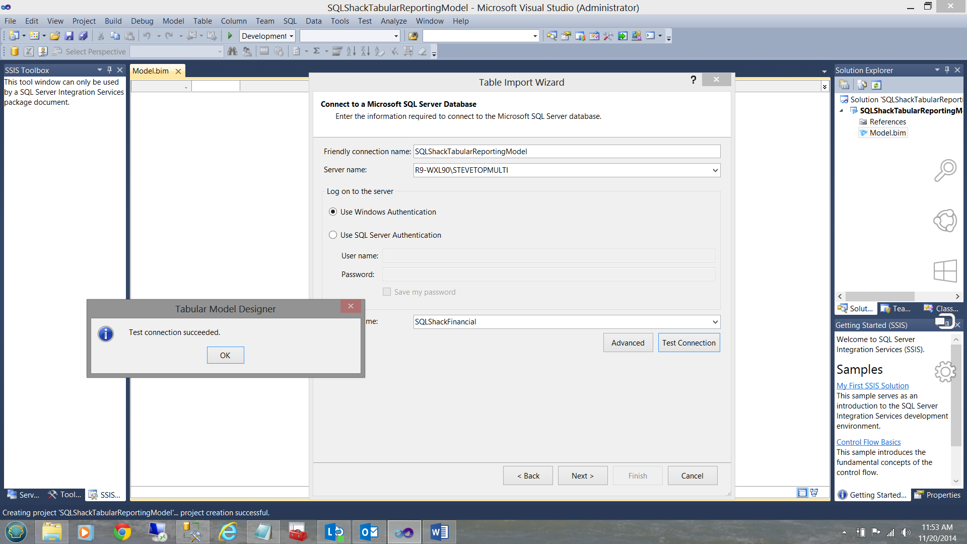
I can now test the connectivity to the ‘SQLShackFinancial’ relational database, the source data for our efforts today.
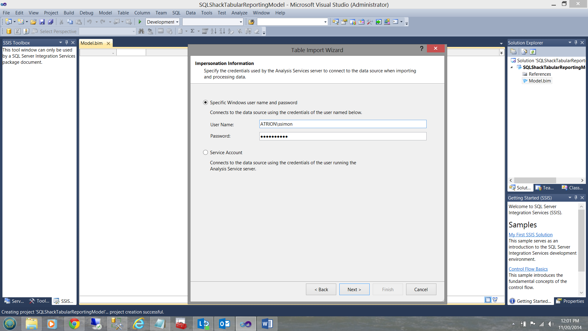
Having defined the connection, I am next asked for the credentials that will be used to access the data (see above). The system then verifies that I have the necessary rights to view the data and if the authentication is successful then the system will ask me to select the table(s) and view(s) that I wish to import into our project (see below).

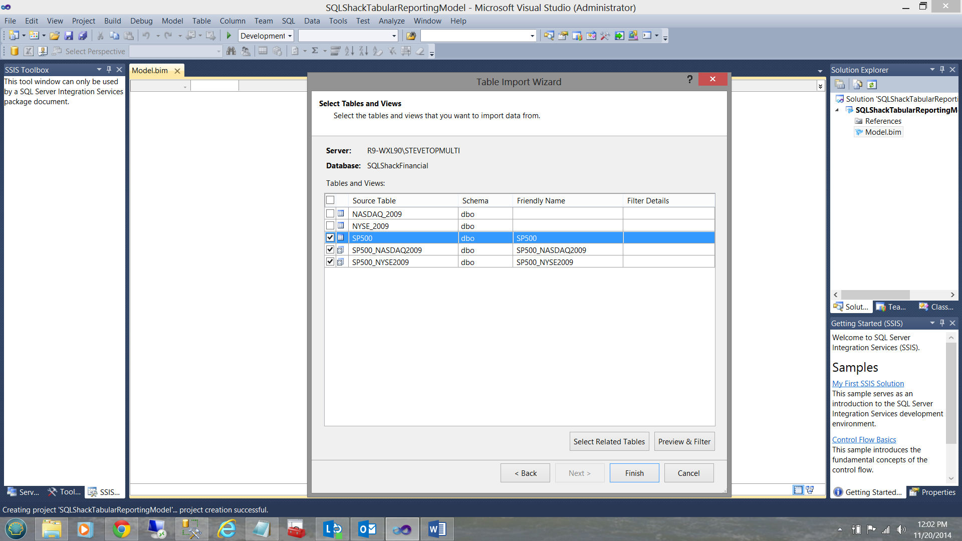
The best ‘fit’ for what we shall utilize in this discussion are data from the SP500 table and from the two views that we created above (see the screen dump above).
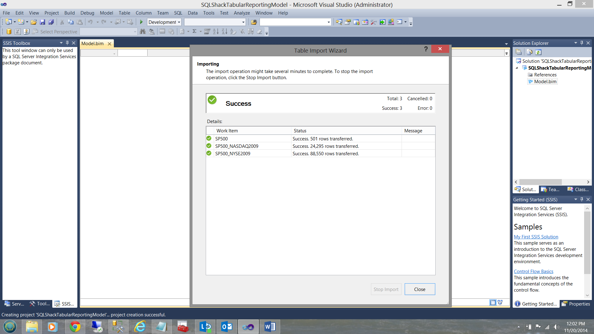
The system now loads the data and when loading has completed (and if the load was successful), you will receive a ‘Success’ notification as may be seen below:
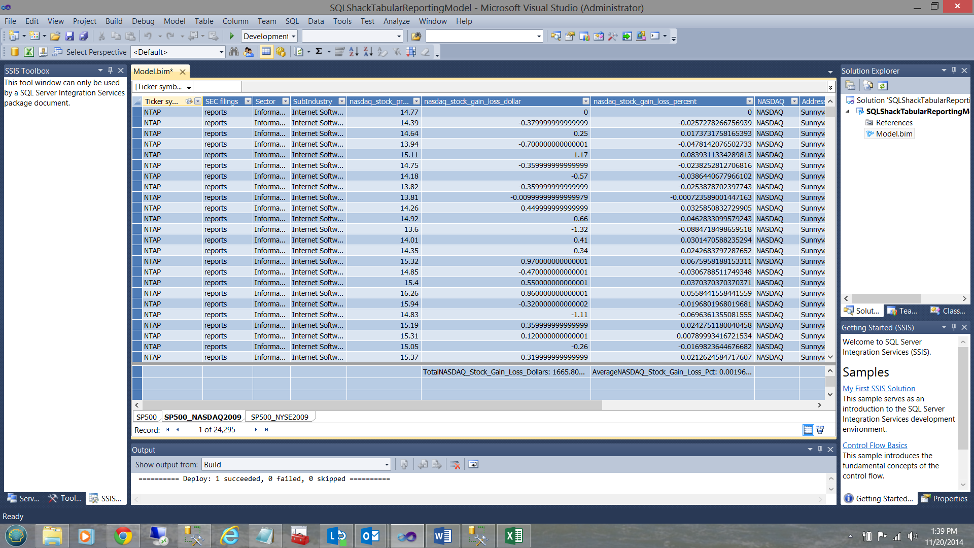
Once the process is complete your screen should be similar to the one below:
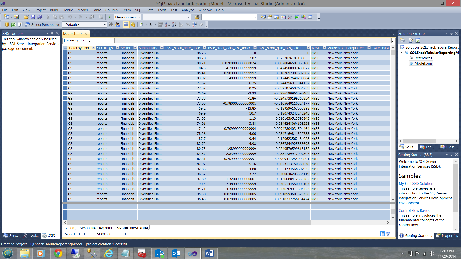
Note that the data from the SP500 table and data from the two views may be seen in the screen dump above. Note also, the manner in which the data is displayed and it does bring to mind the workings of a spreadsheet. This is the big selling point for the product, especially where financial folks are concerned.
Creating our measures
When working with any analytic solution, albeit Multidimensional or Tabular, we have ‘facts’ or ‘measures’ in addition to dimensions. In our case the ‘gain or loss dollars’ and the ‘gain or loss percentages’ are our measures and the sectors and sub-industries will be our dimensions. In short we shall be asking ourselves what are the gain/losses for a particular ‘sub-industry’ within a sector?
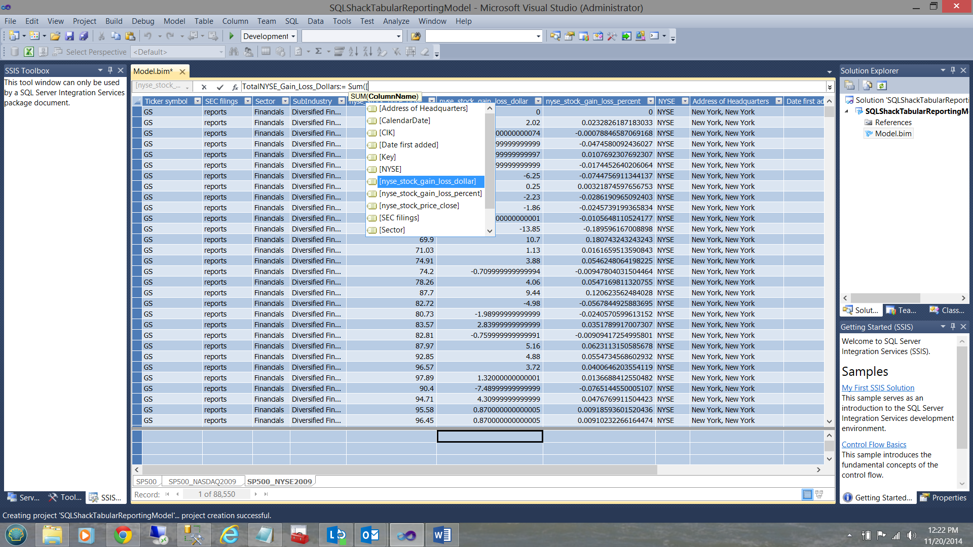
The measures for ‘NYSE_Stock_Gain_Loss_dollar’ and ‘NYSE_Stock_Gain_Loss_percent’ are shown below.
An important point to emphasize is that although at first glance the column/field is merely being ‘summed’, this is NOT the case. What we are in fact looking at is a ‘cube’ and we can utilize our dimensions such as ‘sector’ and ‘sub-industries’ as slicers.
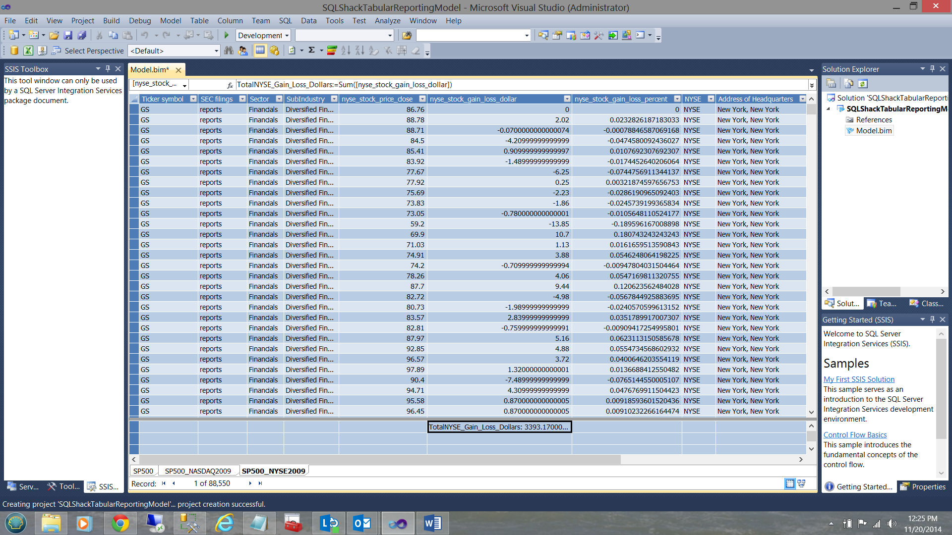
The completed total calculation may be seen below:
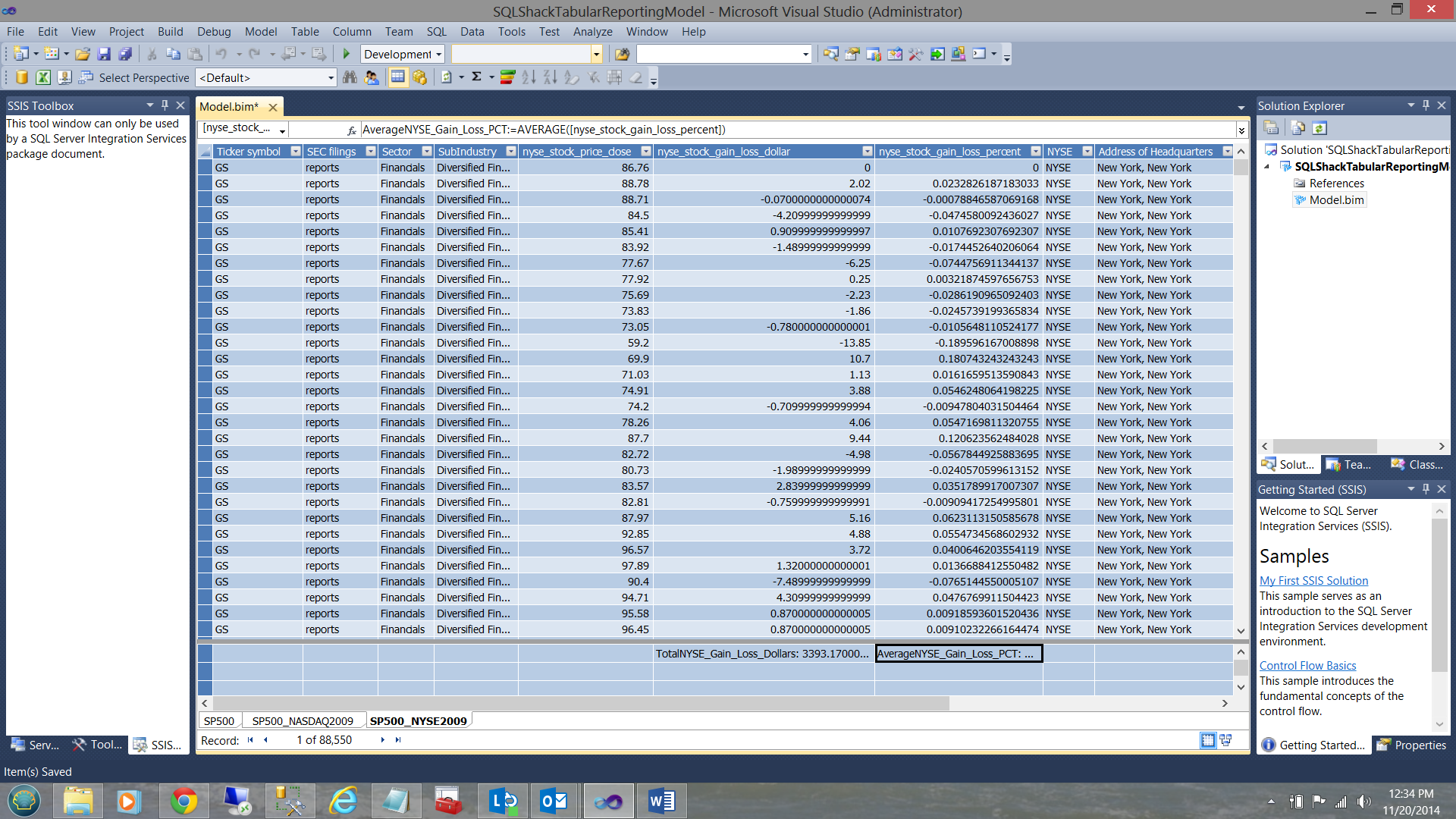
In a similar manner the ‘AVERAGENYSE_Stock_Gain_Loss_Pct ‘field is created (see below).
Using the data from the SP500_NASDAQ view we create similar totals and averages (see below).
Switching over to the relational view (by clicking the icon of ‘three small square boxes’ on the bottom right hand side of the screen containing the grid), we find our ‘Relational’ view.
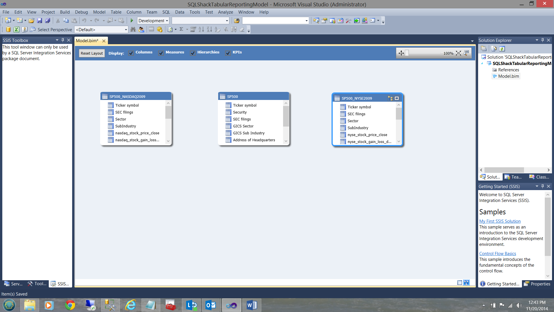
Creating relationships between the table/views
We now ‘join’ the ticker symbol from the SP500 table to the ticker symbol in the SP500 – NYSE2009 view AND link the ticker symbol from the SP500 table to the ticker symbol in the SP500 – NASDAQ view (see below)
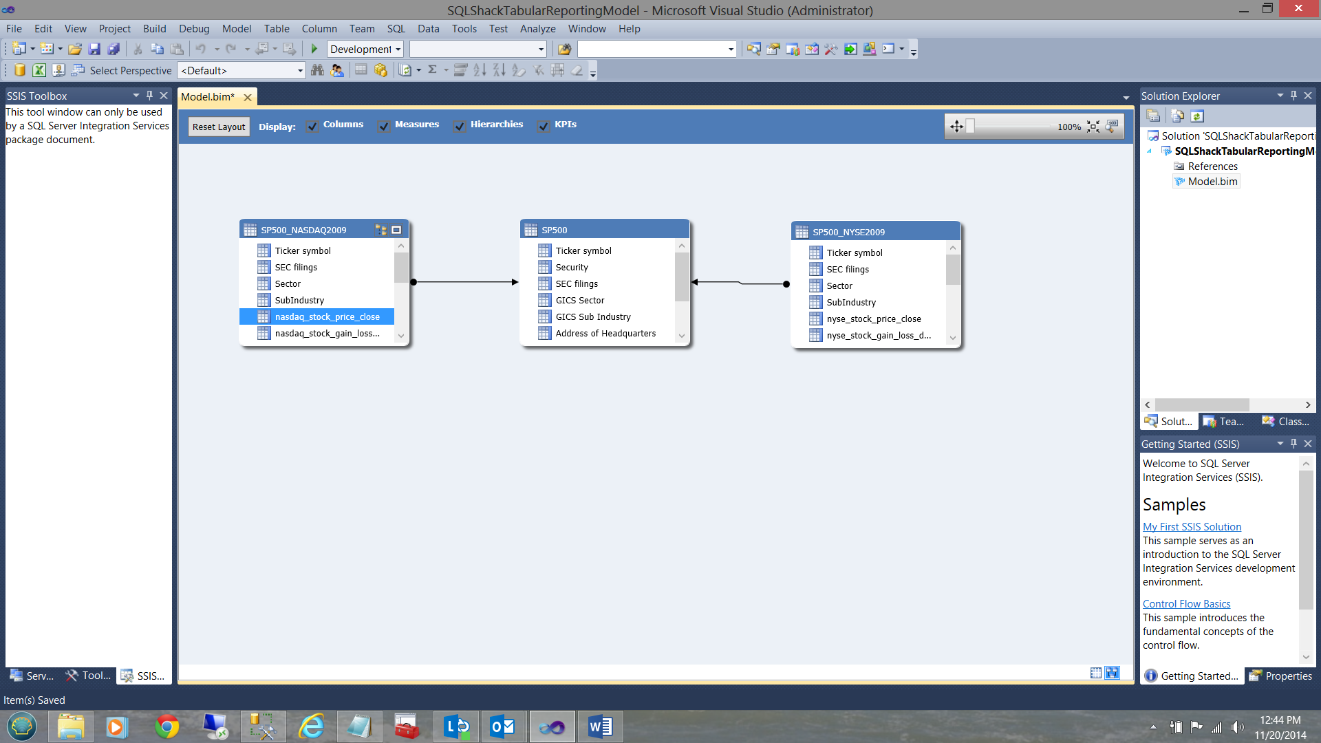
The reader will note that in each of the tables / views (shown above), that there is a ‘sector’ and ‘sub-industry’ field. Sectors have ‘babies’ called sub-industries. What we need to do is to create a hierarchy on each of the tables / views (shown above) shown above.
We first right click on the SP500-NASDAQ entity. The context menu appears.
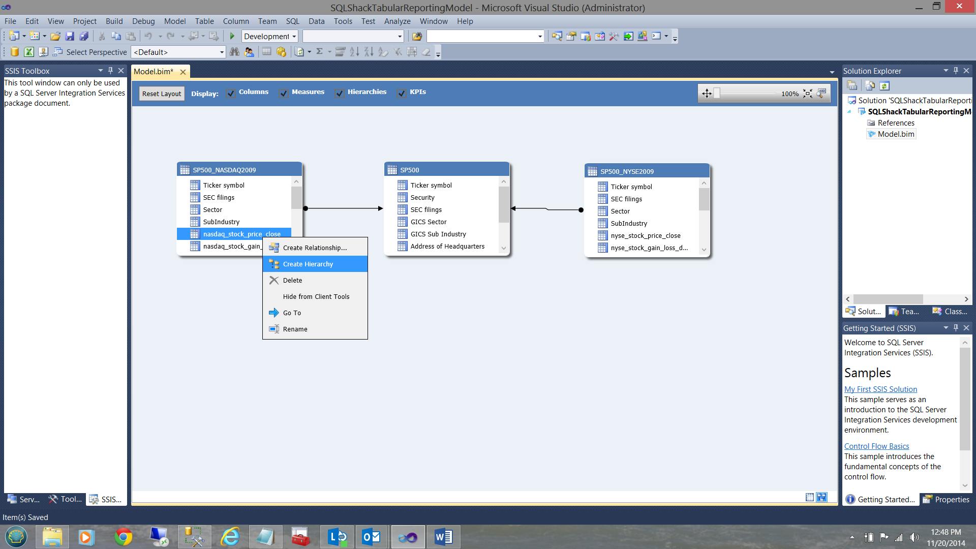
I choose ‘Create Hierarchy’. Note that a ‘hierarchy’ has been established in the screen dump below:
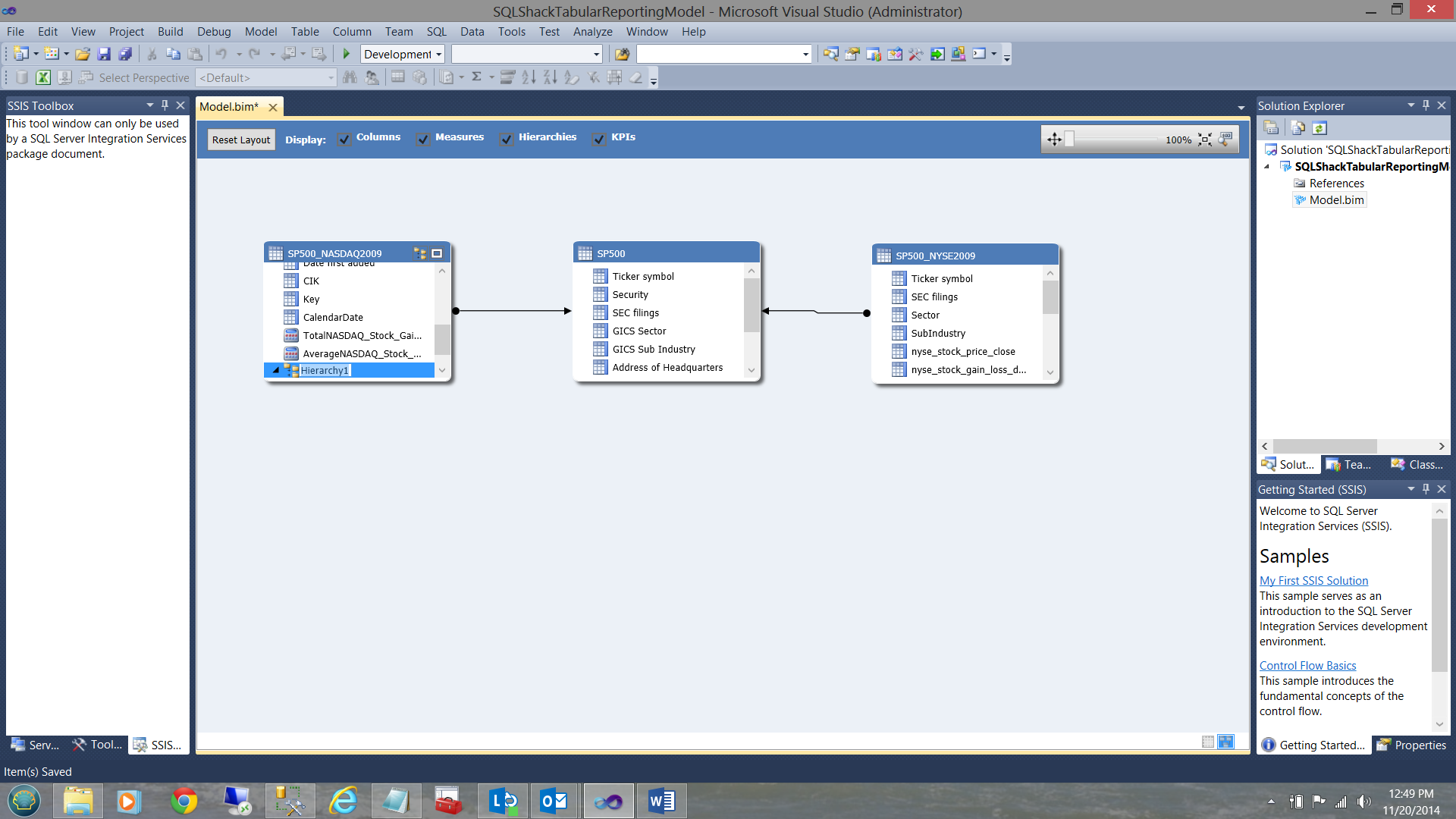
I rename the hierarchy and drag the sector and sub-industry fields into the hierarchy (see below).
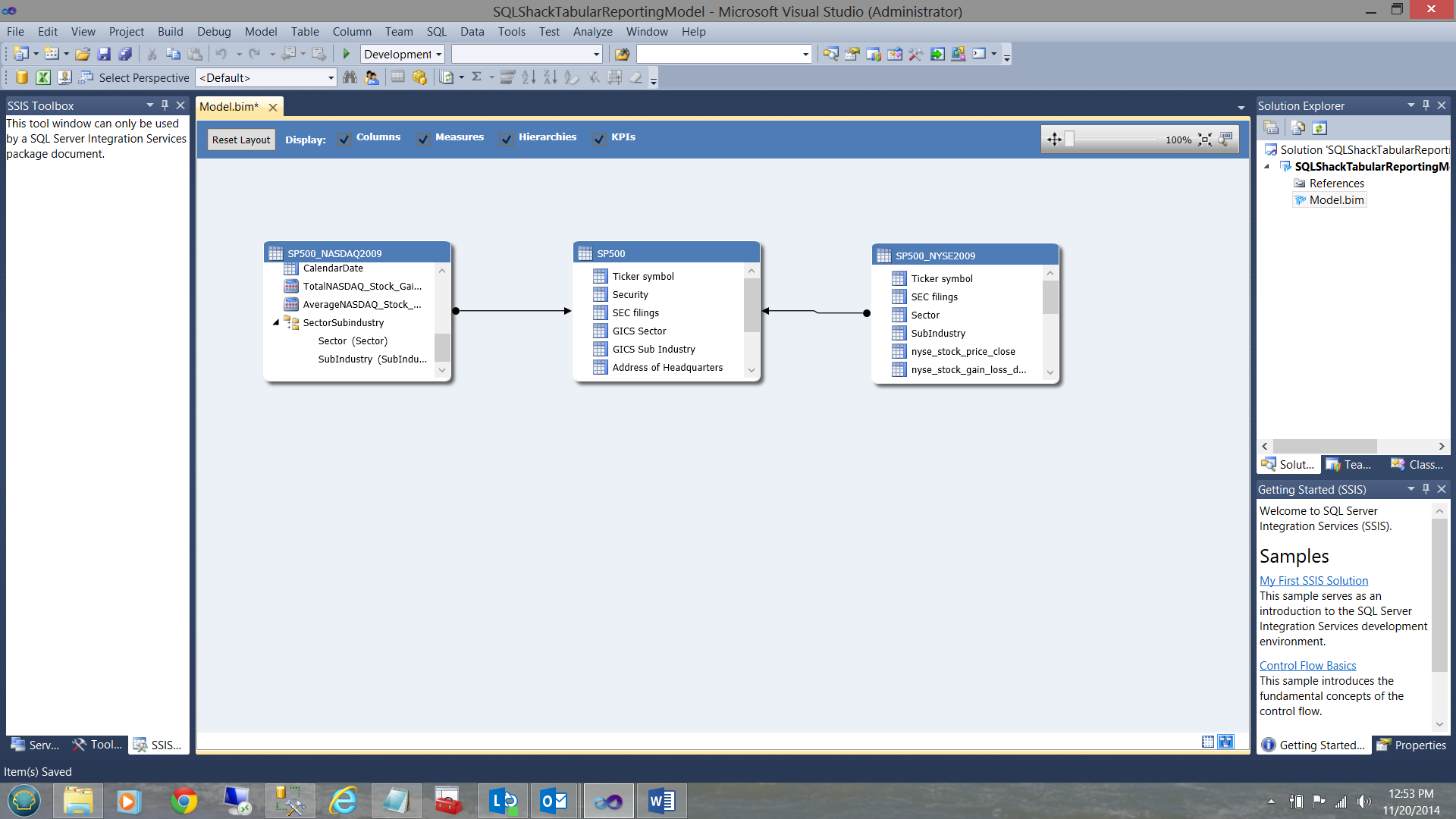
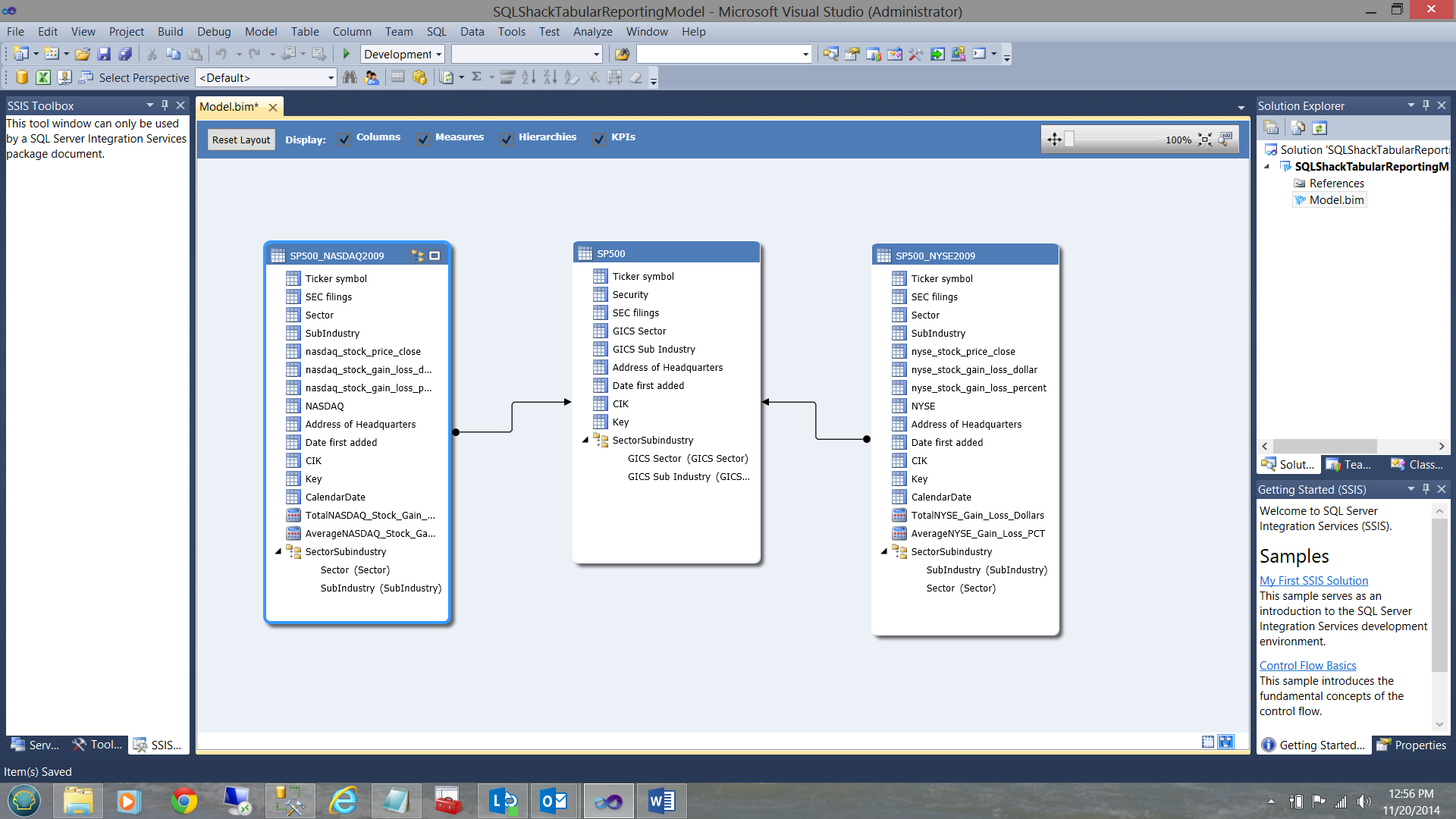
In a similar manner, I create the hierarchy for the SP500 entity and for the SP500-NYSE2009 entity (see below).
We are now ready to deploy our project.
Deploying our project
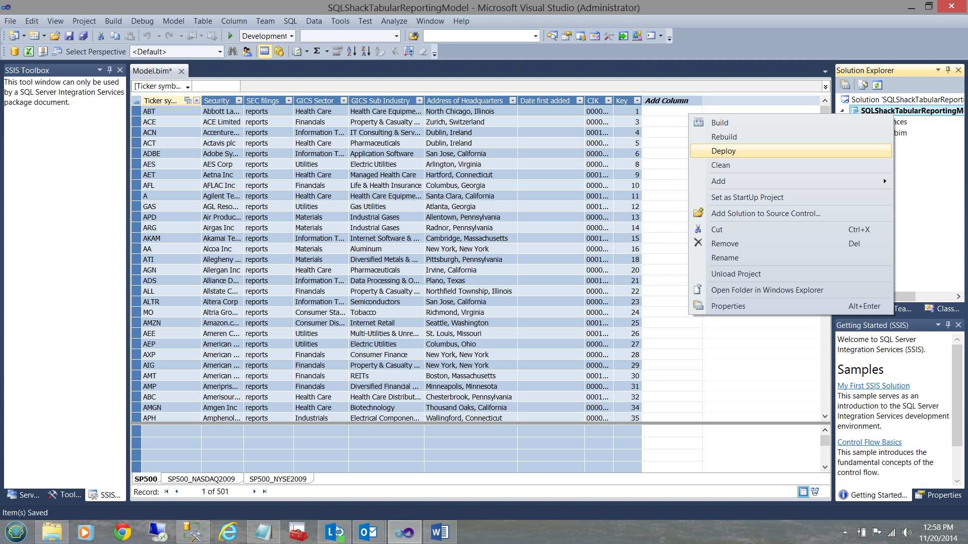
I right click on the ‘SQLShackTabularReportingModel’ and select deploy (see above). Upon successful completion of the deployment, you should receive a screen similar to the one shown below:
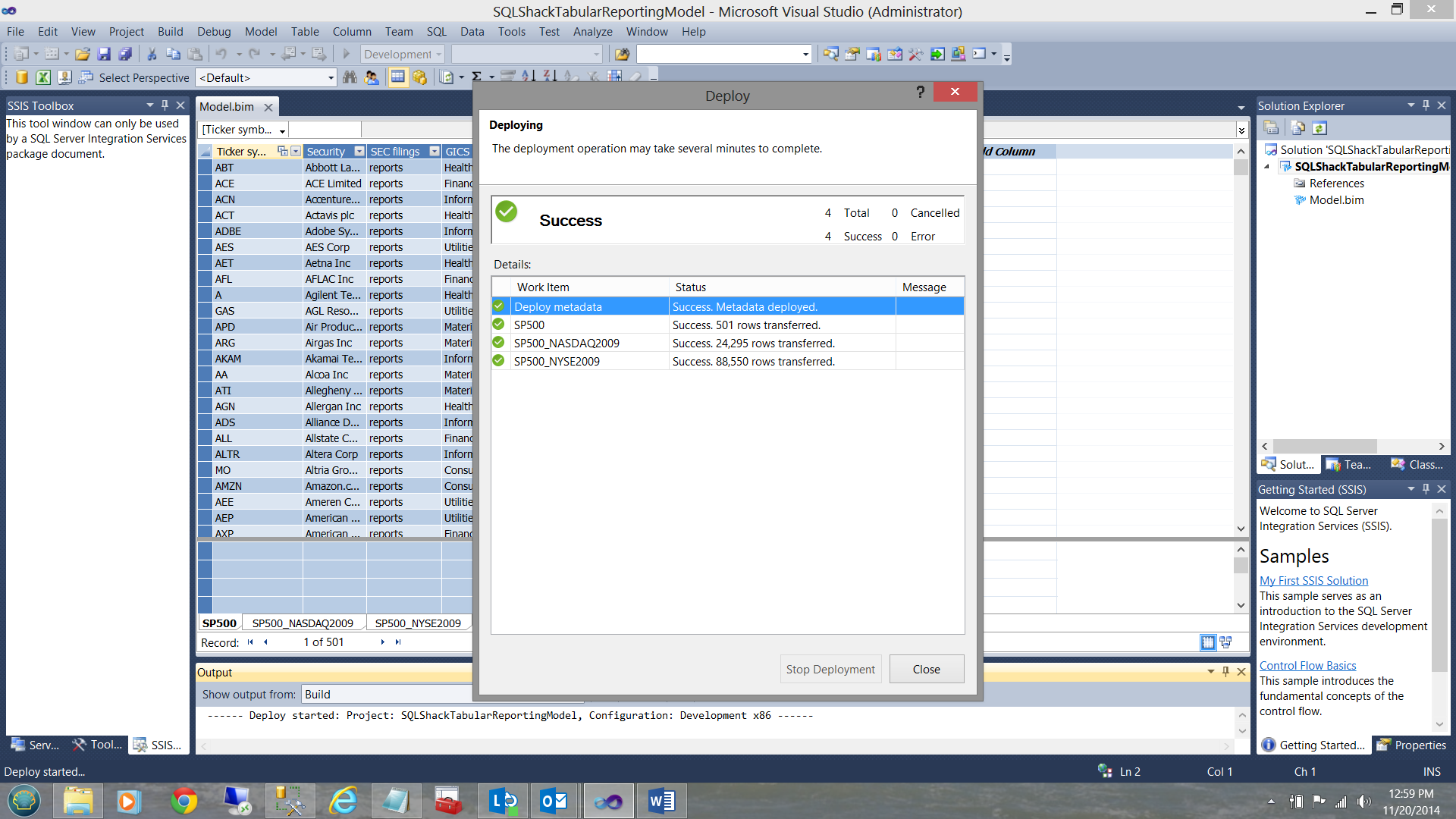
Our work here is now complete. Let us see what we have done!
Meanwhile back in Analysis Services
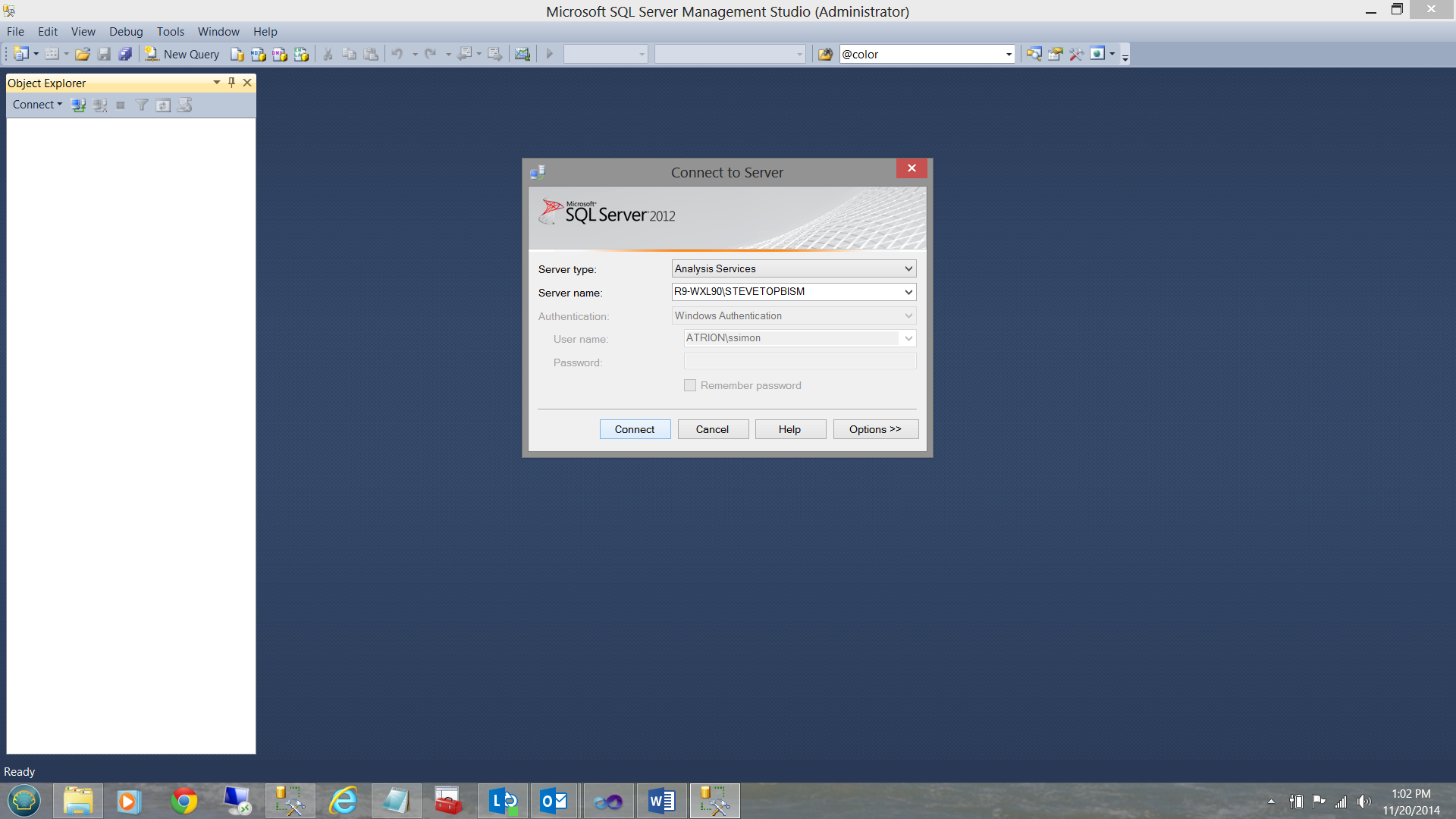
In order to have a quick look at what we have just created, we bring up Analysis Services.
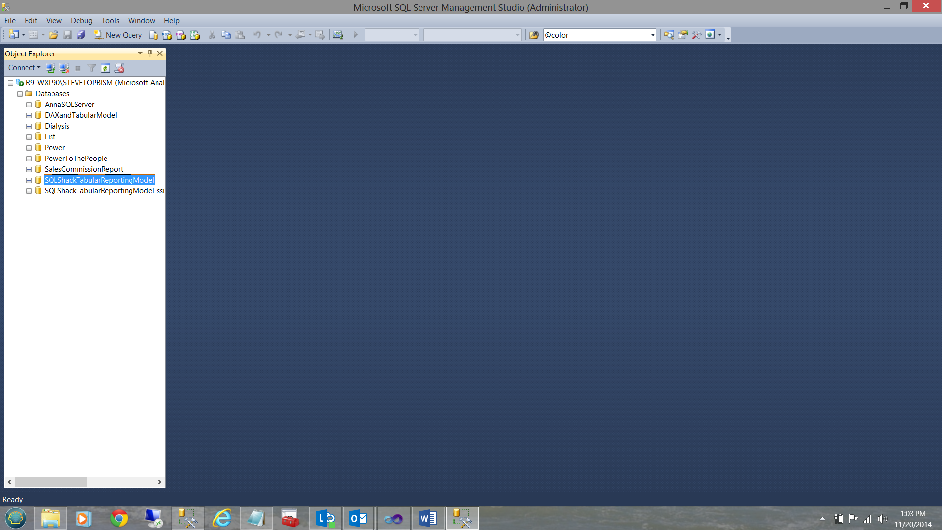
Once in Analysis Services, we can see the database that we just created.
Now that we know that our deployment was successful, we are now ready to create a few reports!
The proof of the pudding is in the eating!
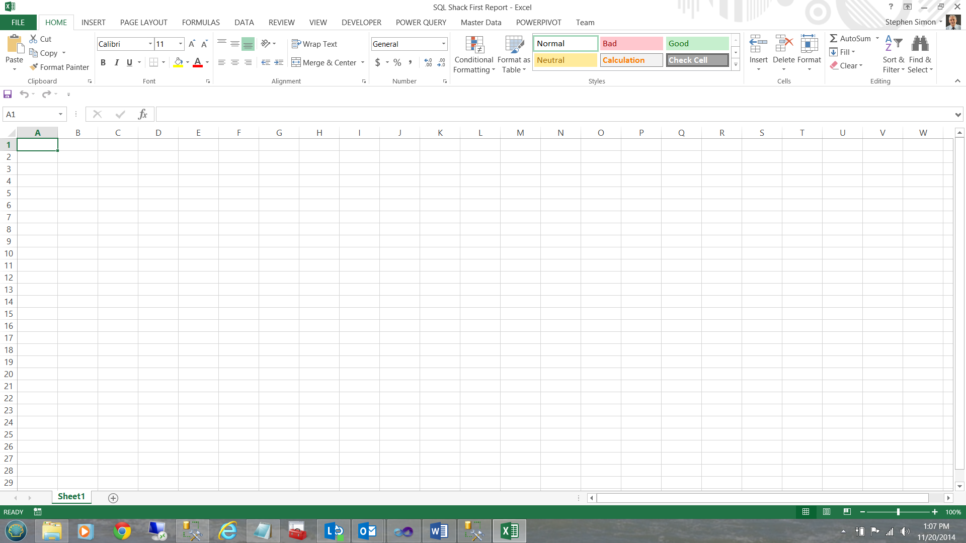
As mentioned within the introduction, our client utilized Excel as a GUI. With this in mind, our reporting today will be via Excel.
Having opened Excel we begin with a new workbook.
Our first task is to create a data connection to our newly created tabular model.
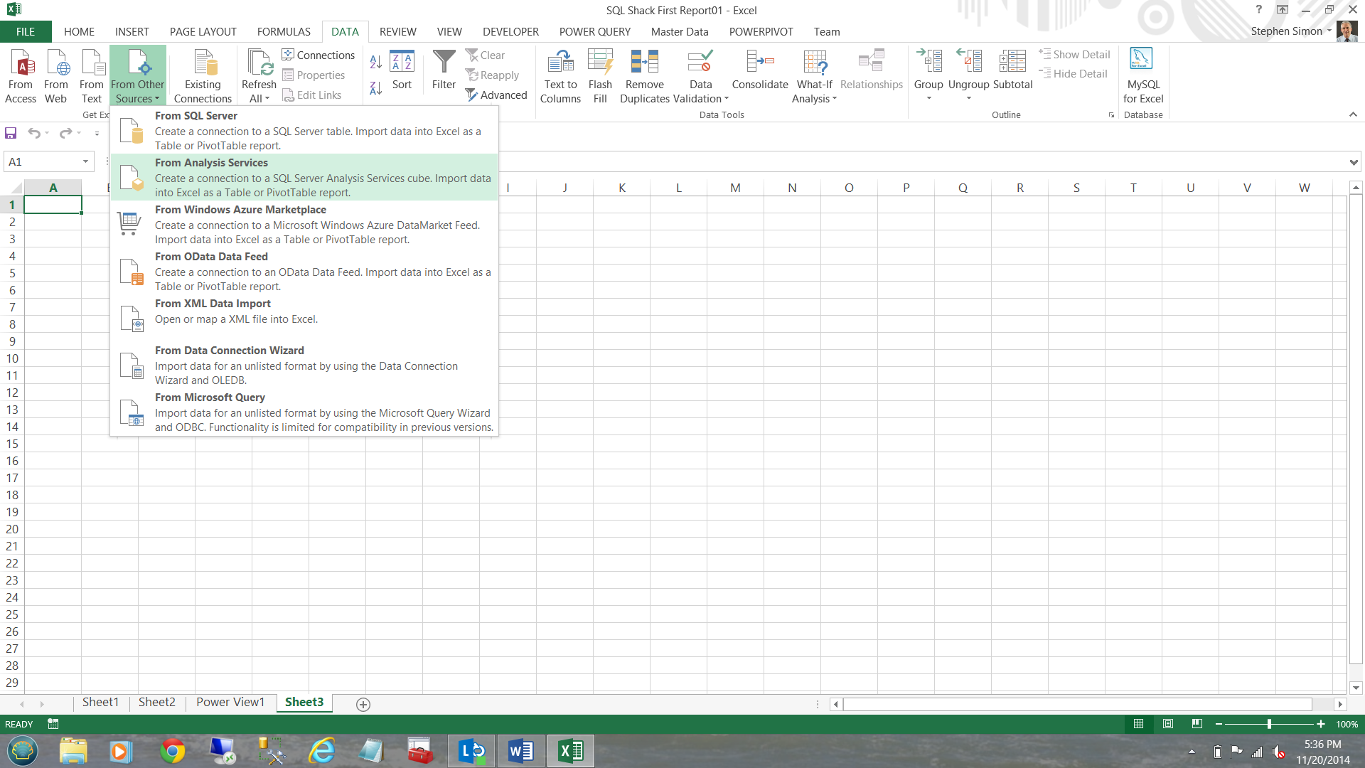
I click on the ‘Data’ tab and select ‘From other sources’ (see below).
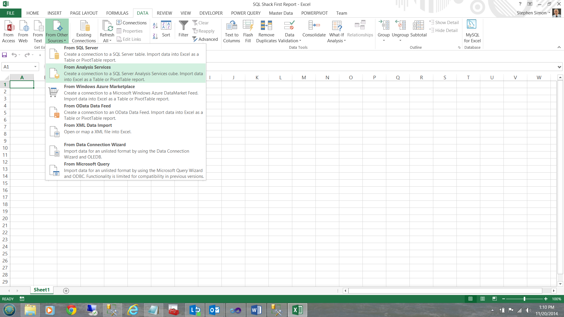
I choose ‘From Analysis Services’
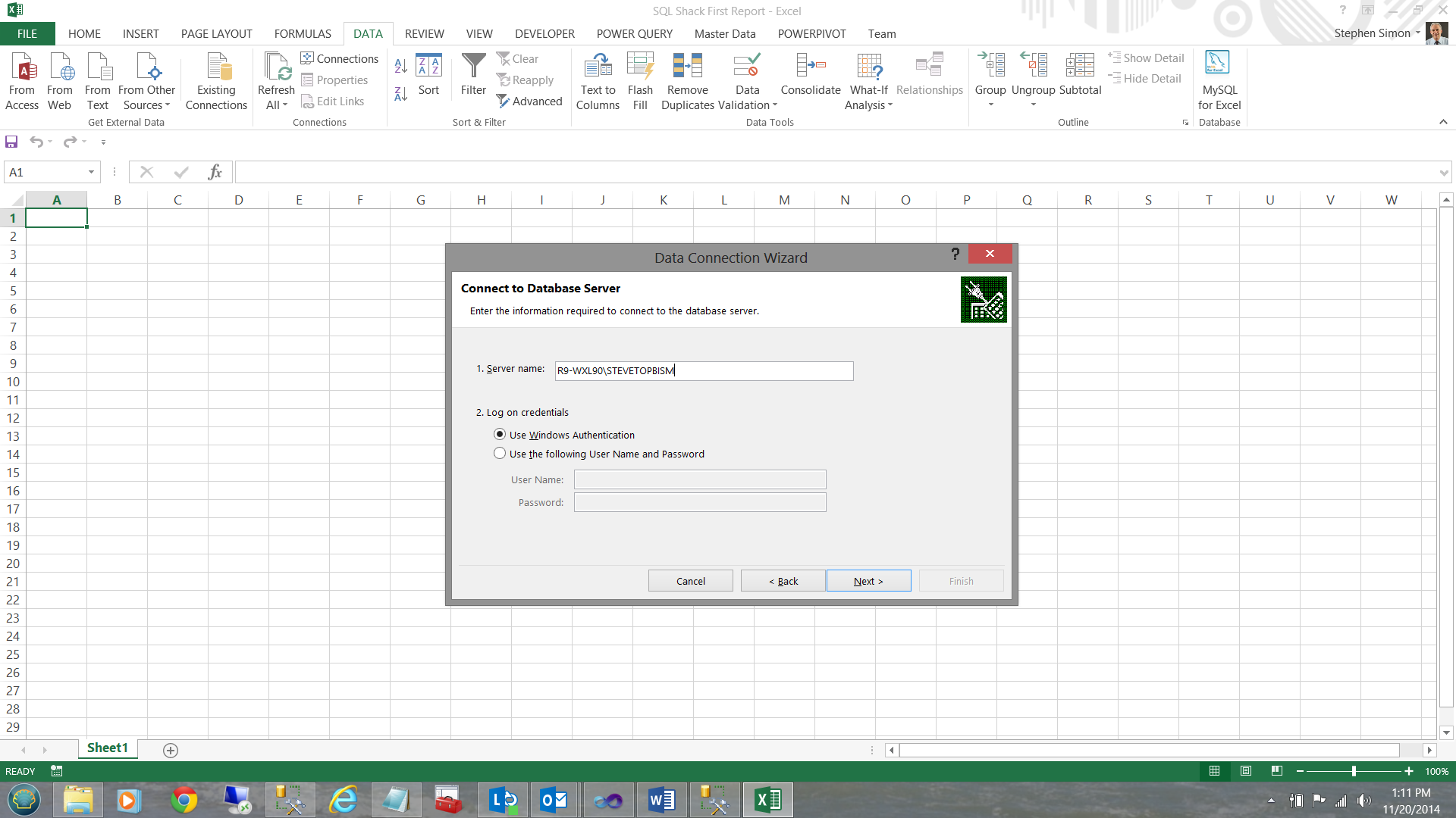
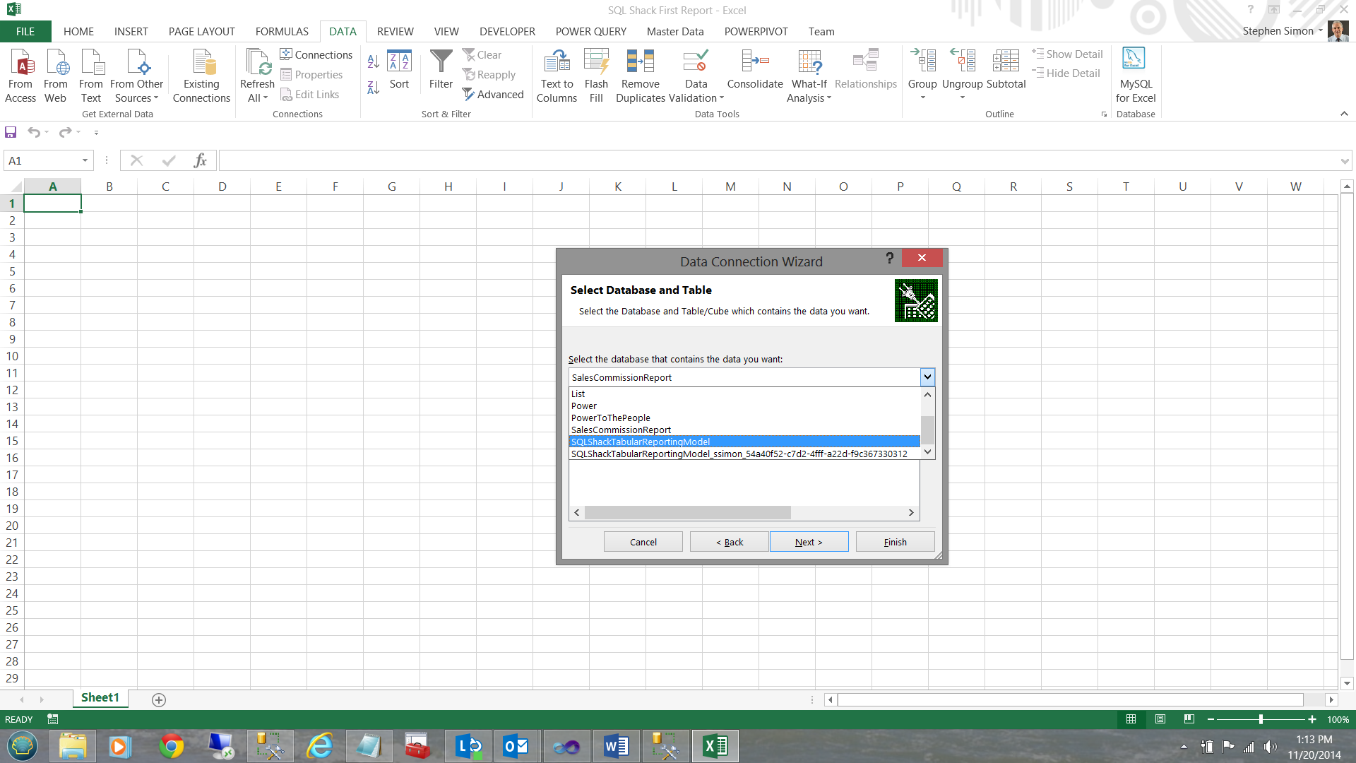
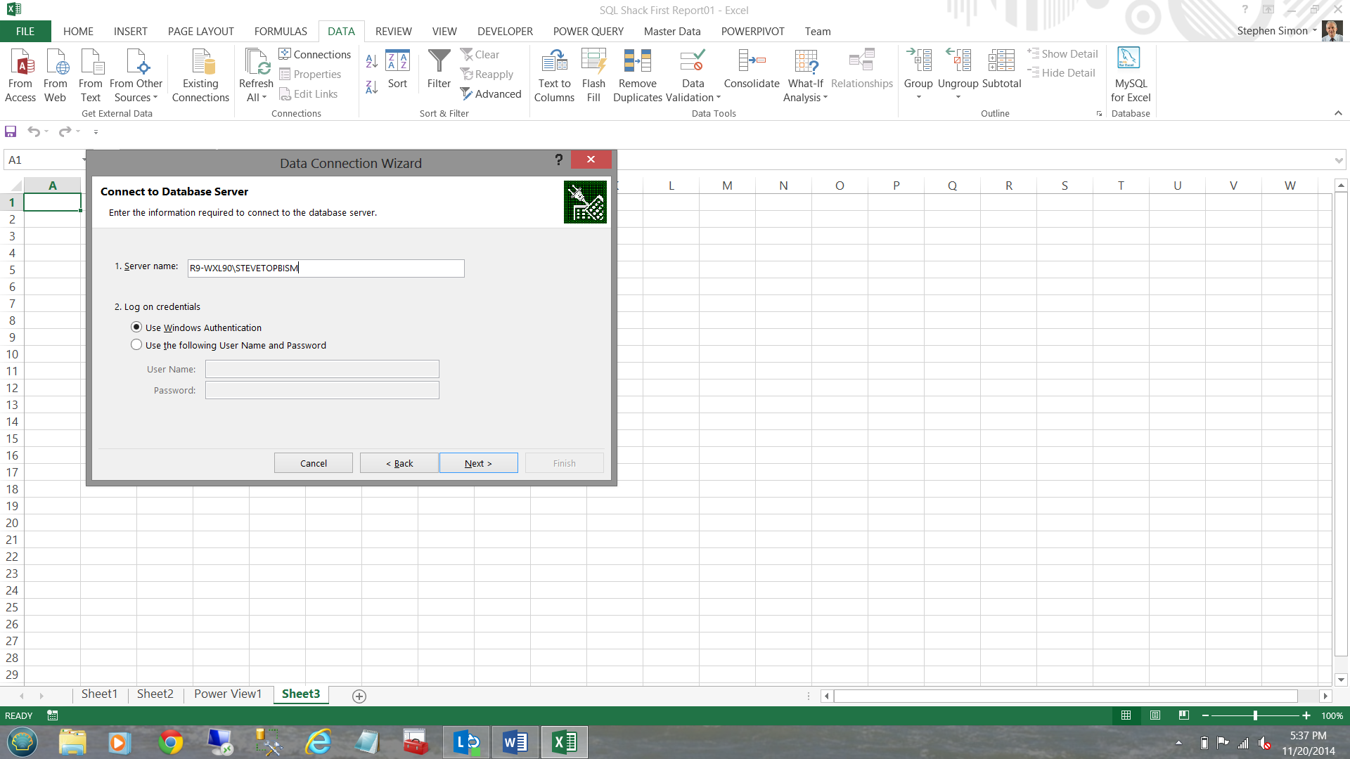
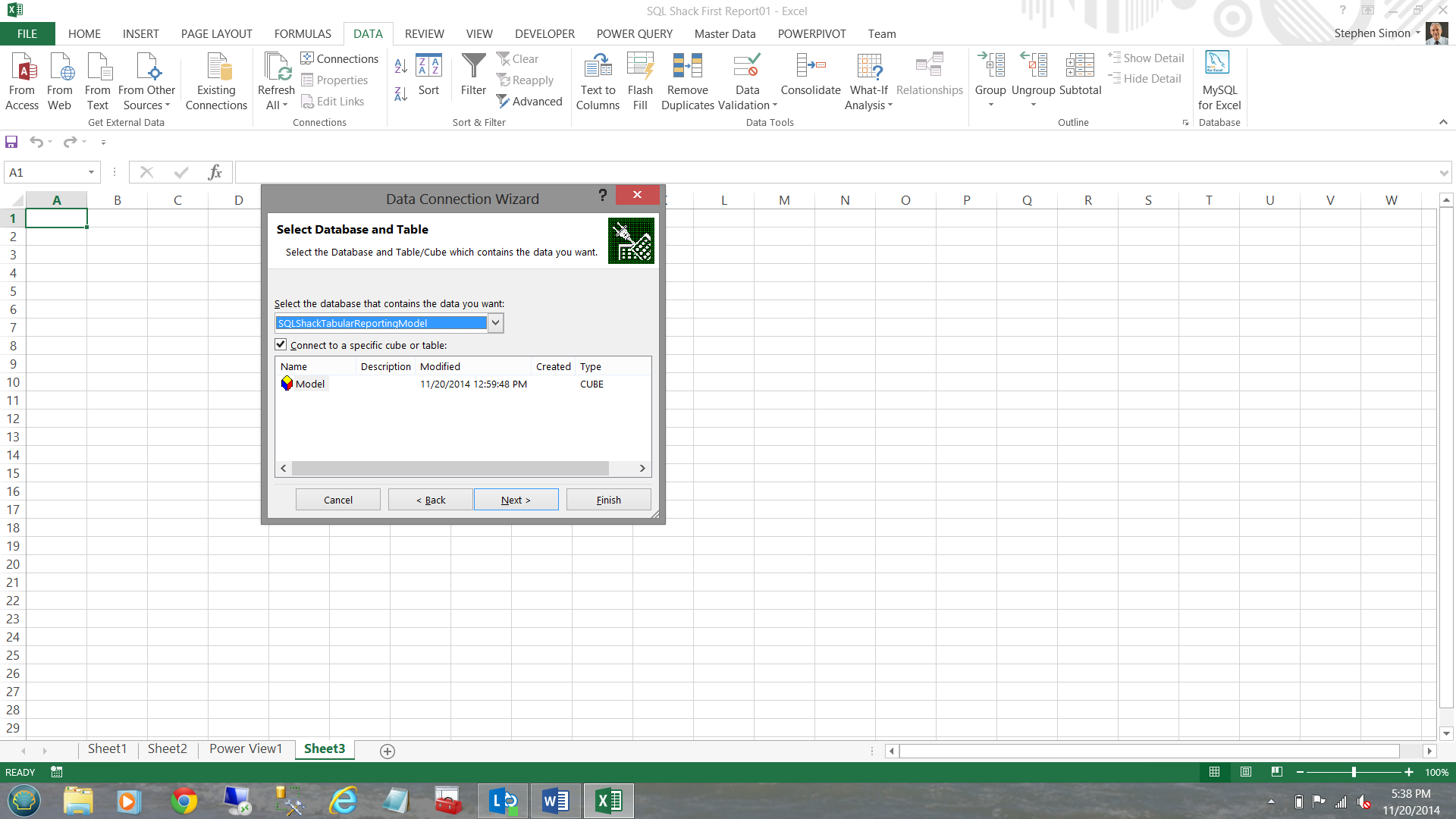
I now let Excel know which server contains the data and I select windows authentication for my credentials (see above). I then click ‘Next’. I shall now select our ‘SQLShackTabularReportingModel’ database (see below).
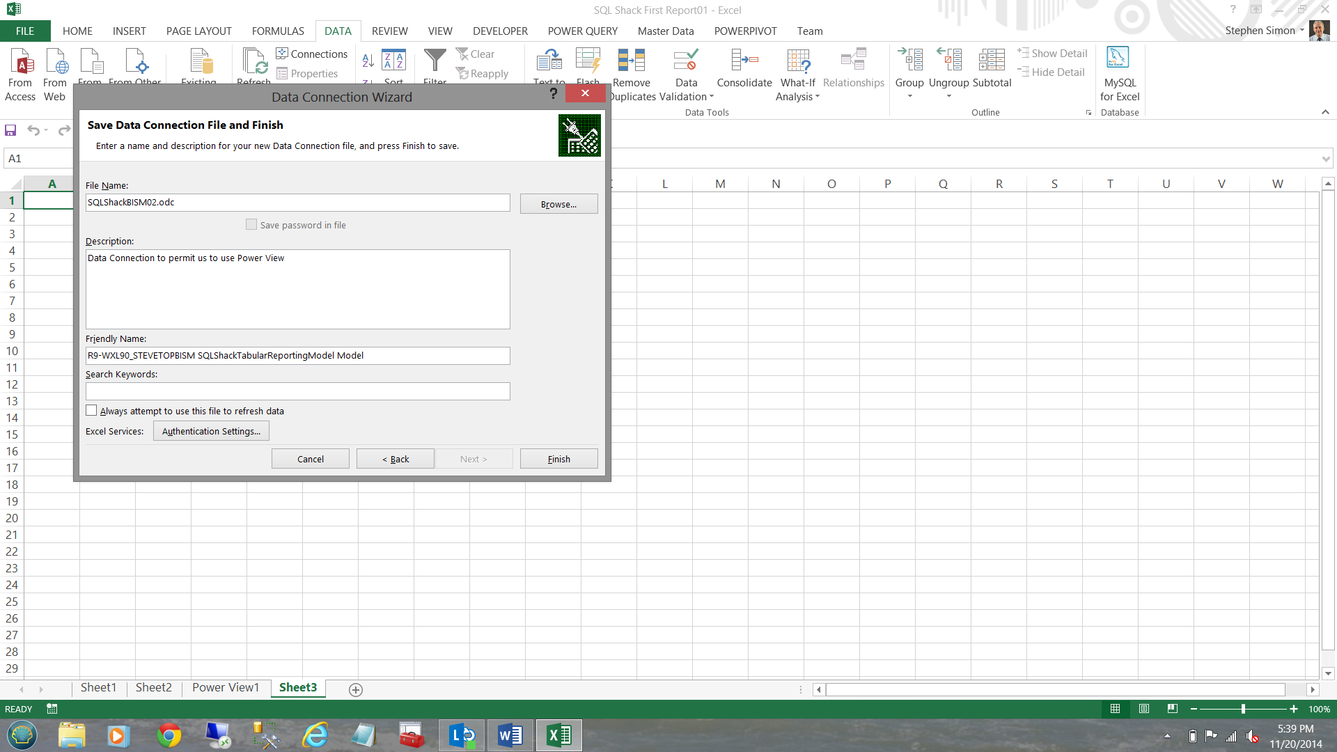
Whilst I have defined which database I wish to use, I must still create a connection from Excel to that database before I can work with the data. This is achieved via a ‘Connection File’.
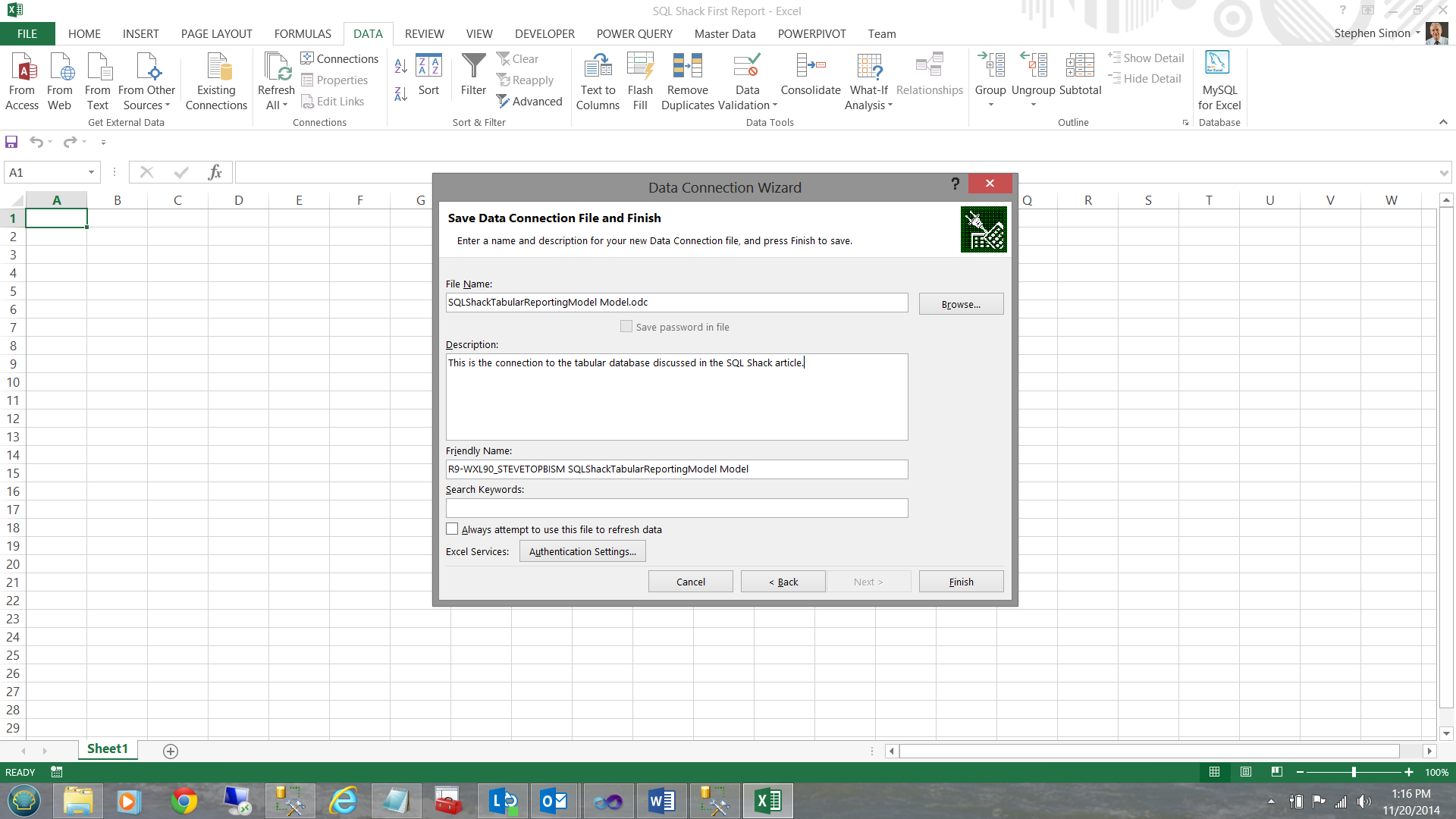
I must now give a name to our connection file. I also give the connection file a meaningful description so that the next time that I am looking for it, it will be come immediately apparent that this is the connection for which I am looking.
I click ‘Finish’.
This done, Excel wishes to know if I would like to a PivotTable report. I click OK (see below).
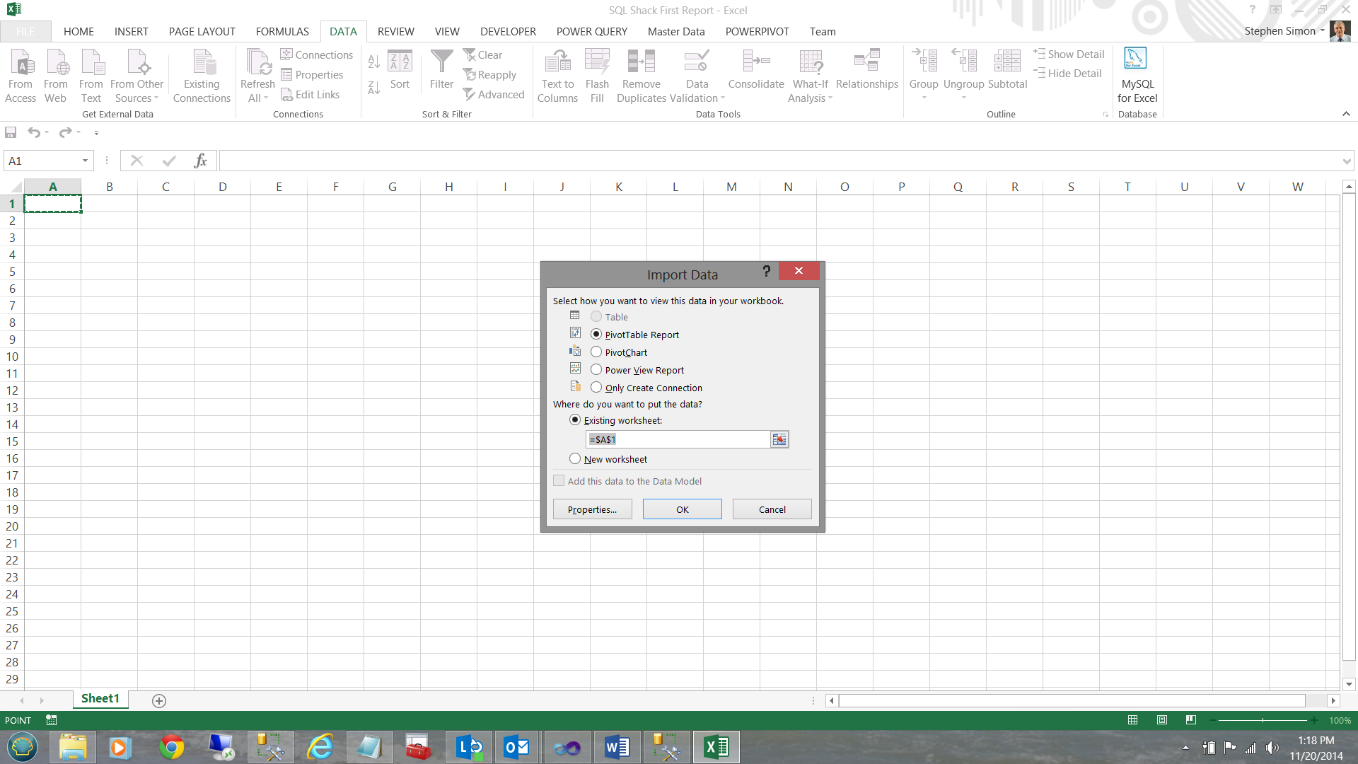
Having clicked OK, we find ourselves within a ‘PivotTable Report’, with the cells marked ‘Pivot Table1’ being where all of the ‘magic’ occurs.
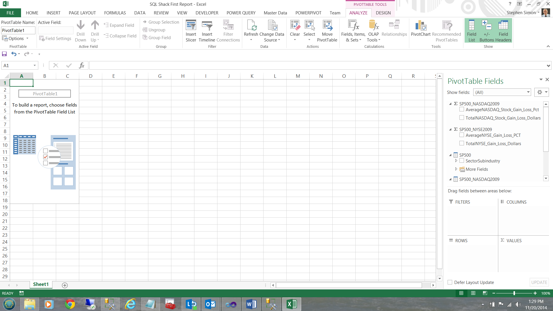
After examining the ‘PivotTable Fields’, note that the summary fields (which we created in the BISM model) are visible in the center right of your screen.
These summary fields are denoted by the Greek letter Sigma Σ
Selecting the SP500_NASDAQ summations, our screen immediately changes (see below).
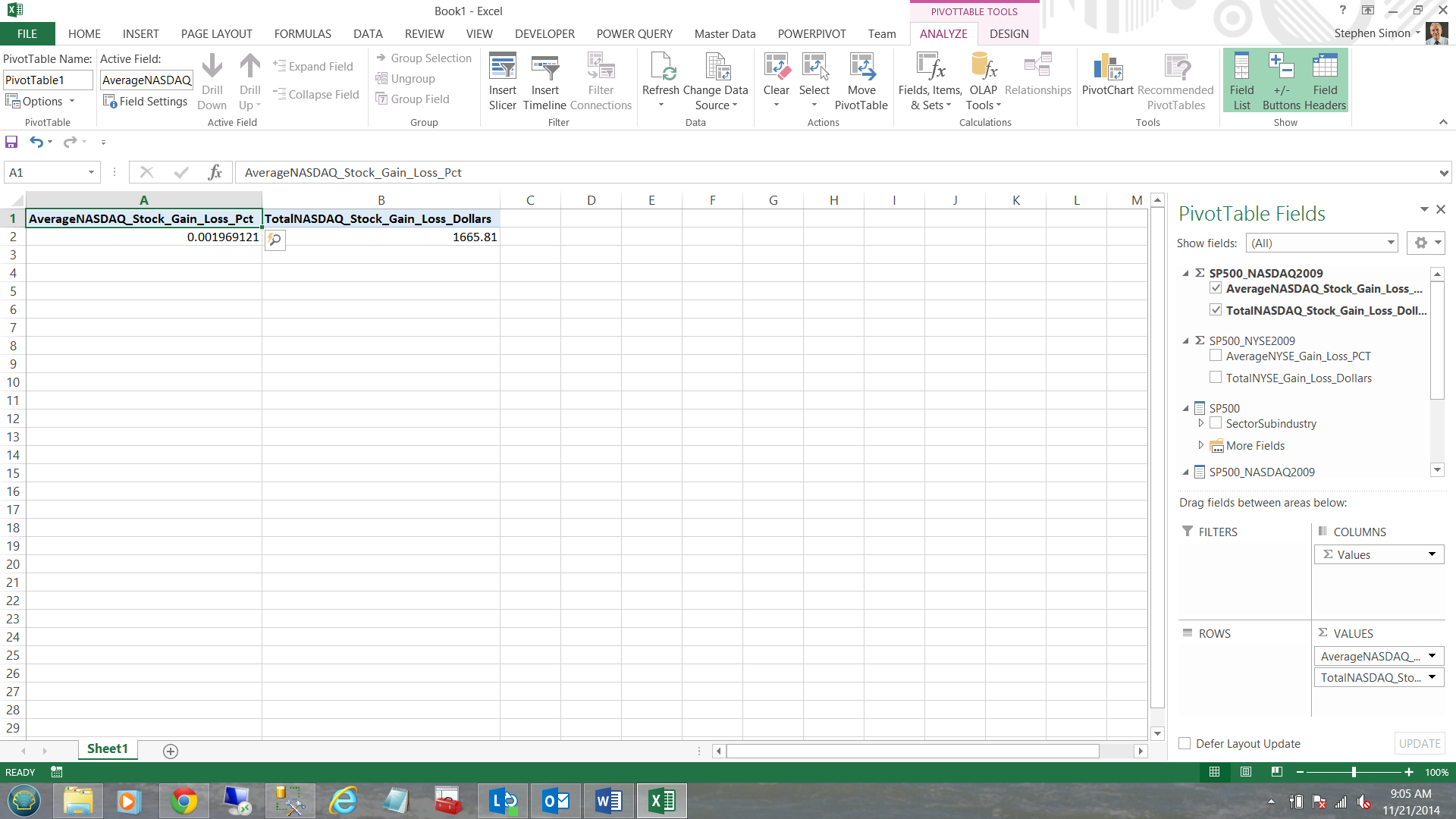
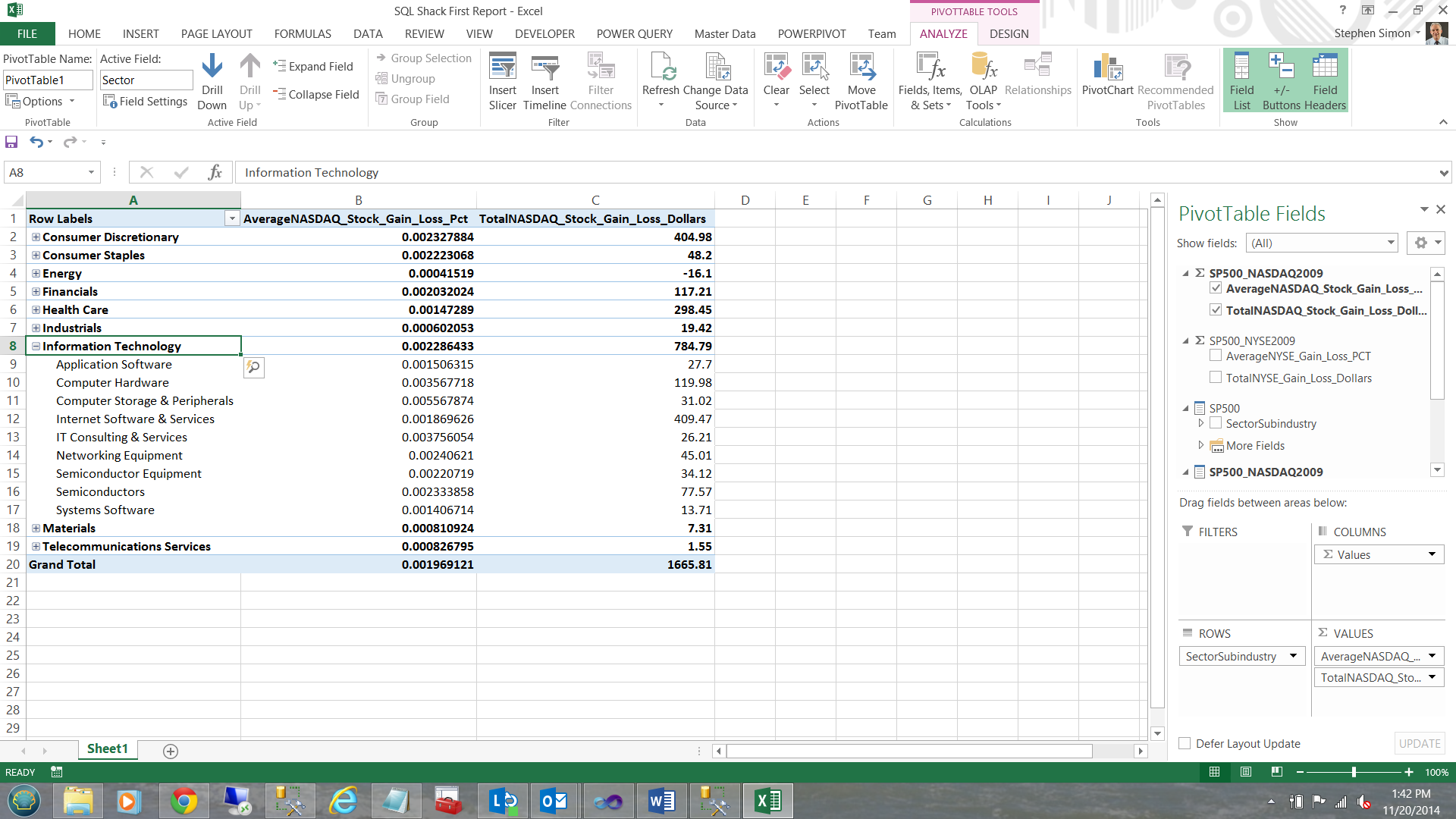
Note that this is a summation of all records within the entity. What we really want to do is to look at the data in a more granular manner fashion; therefore I now ‘check’ the ‘SectorSubindustry’ hierarchy which is then brought onto our work surface. We now have a clear view of the data 🙂 (see below).
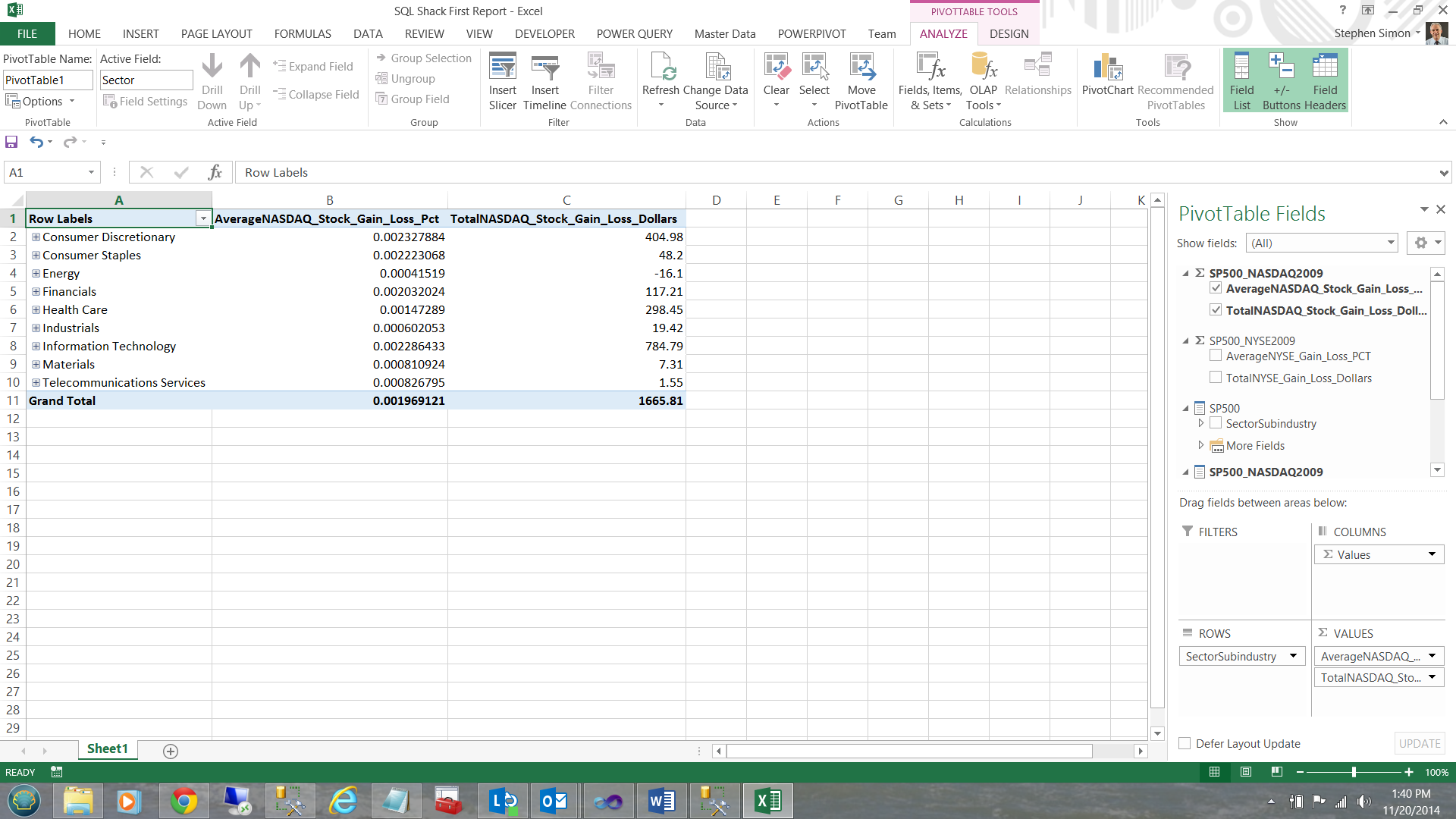
Drilling through… we now find that ‘Information Technology’ has a slew of sub-industries. I click on the + sign next to ‘Information Technology’.
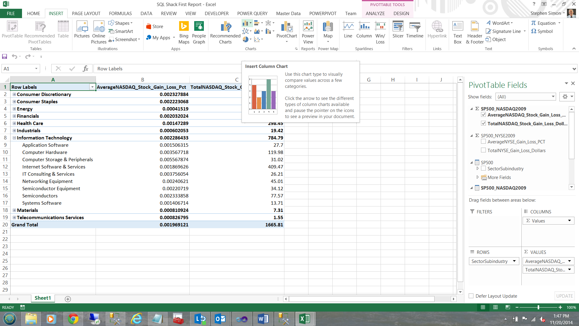
Last, but not least, let us add a chart to our PivotTable Report. Placing my cursor in one of the cells in column A, I click ‘Insert’ and choose ‘Chart’ and then ‘Insert Column Chart’ (see below).
Without any further interaction, a chart is created based upon the data that we have.
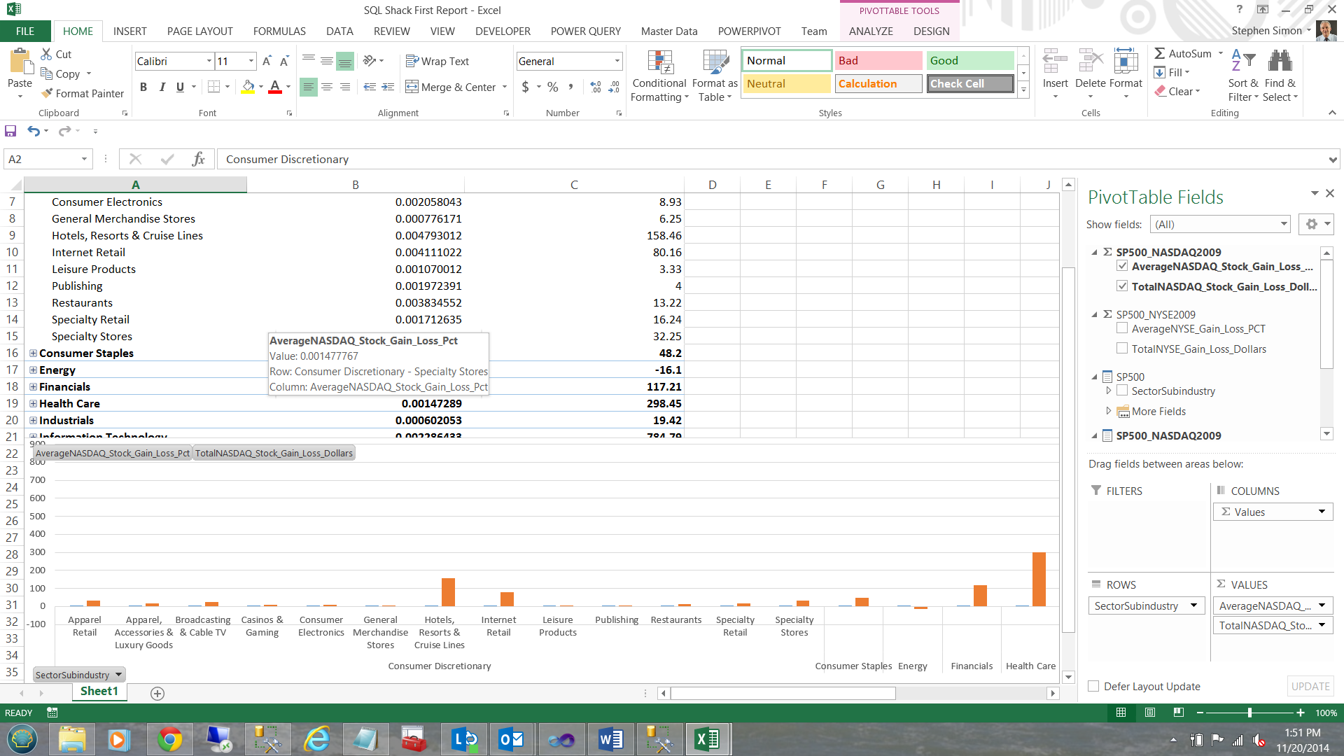
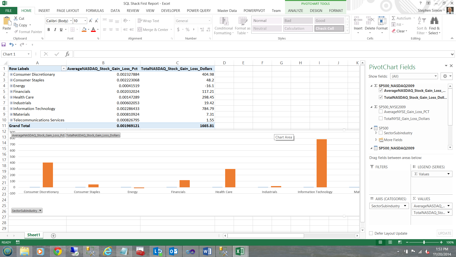
The astute reader will note that our chart is showing the sub industry data BECAUSE we have the ‘Consumer Discretionary’ tab exploded. Closing ‘Consumer Discretionary’ causes the chart to show sector related values (see below).
Now, how cool is this!!!
Moving on:
In a similar fashion we could create a SP500 – NYSE Pivot Report.
Creating our second report, this time via Power View
Power View is similar to Power Pivot except that it permits more ‘bangers and whistles’ to be added to the report. In the world of ‘Vanilla’ this is ‘Strawberry’.
To create our first Power View Report, we open up a new sheet within our workbook.
Once again we choose Data, ‘From Other Source’ and then ‘From Analysis Services’.
We now tell Excel where the data is located (see above) and click next.
Once again, I select our SQLShackTabularReportingModel (see above) and click next.
I name our second connection differently to avoid conflicts should I wish to use the first connection again. I then click ‘Finish’.
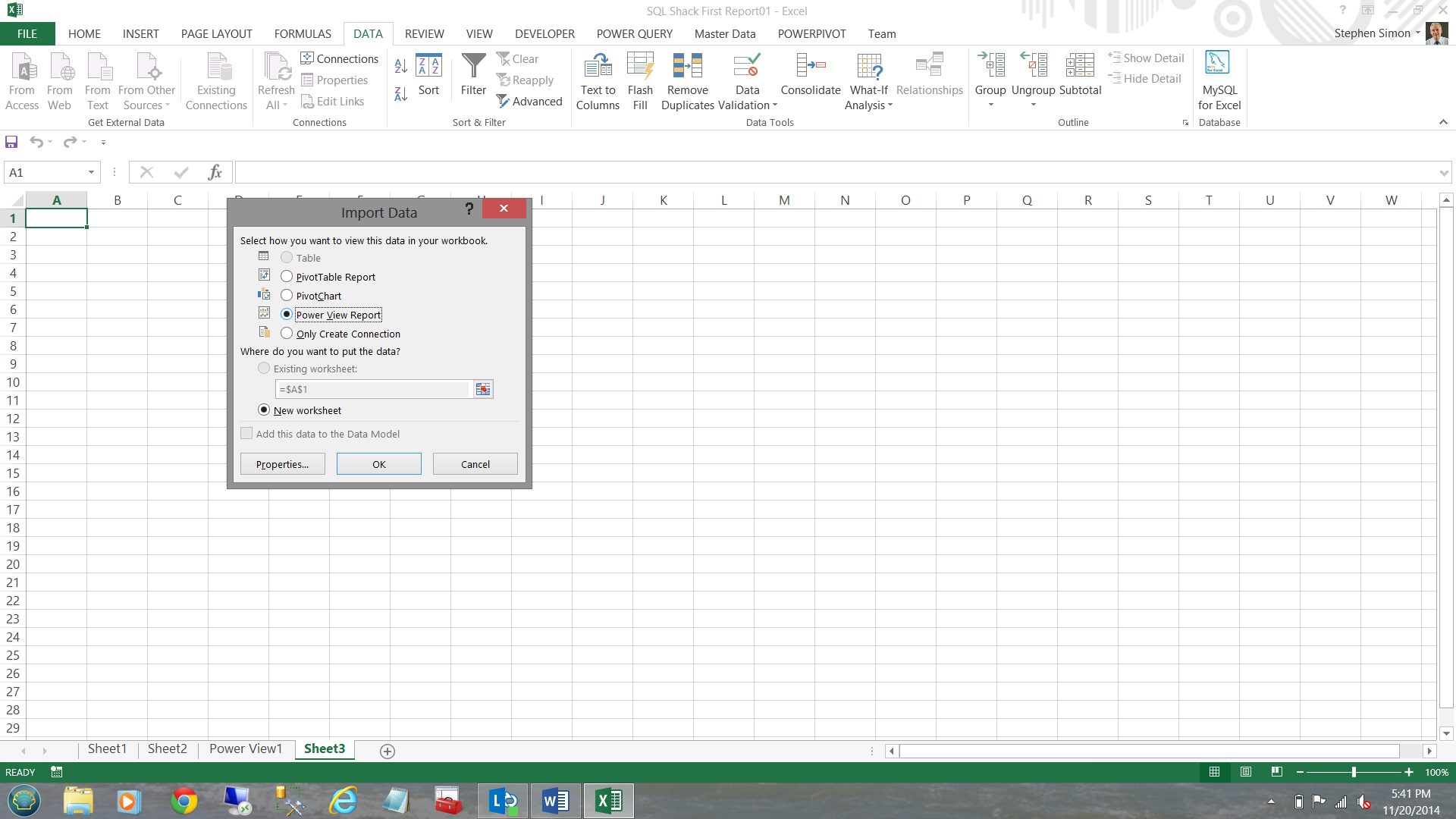
The reader will note that the same ‘Import Data’ dialogue box appears HOWEVER this time I choose create ‘Power View Report’ (see below).
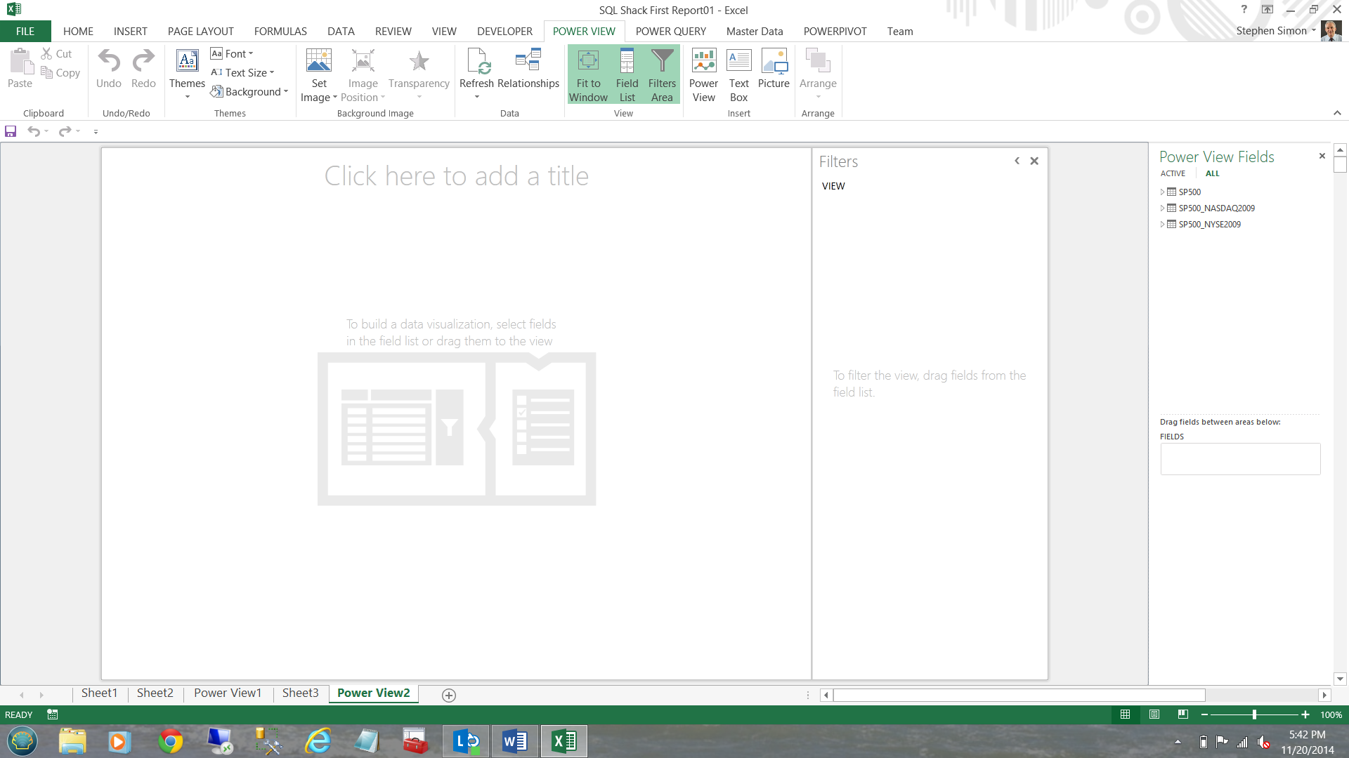
We are now taken to our ‘Power View Design’ screen. Note that the data entities from our SQL Server BISM project are waiting for us, on the right hand side of the screen.
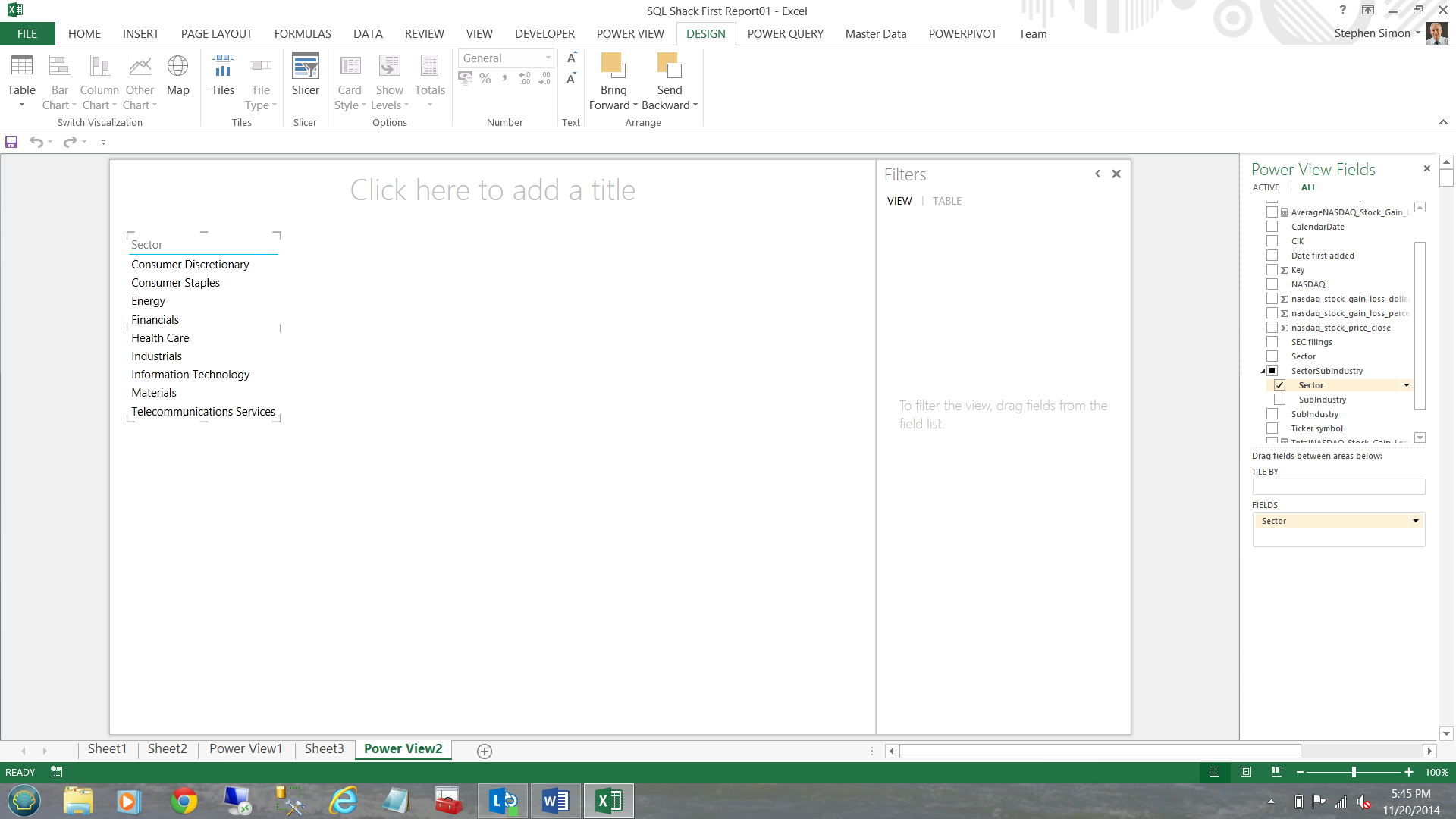
Opening the SP500 – NASDAQ entity, I add the sector from the dimension fields (see below).
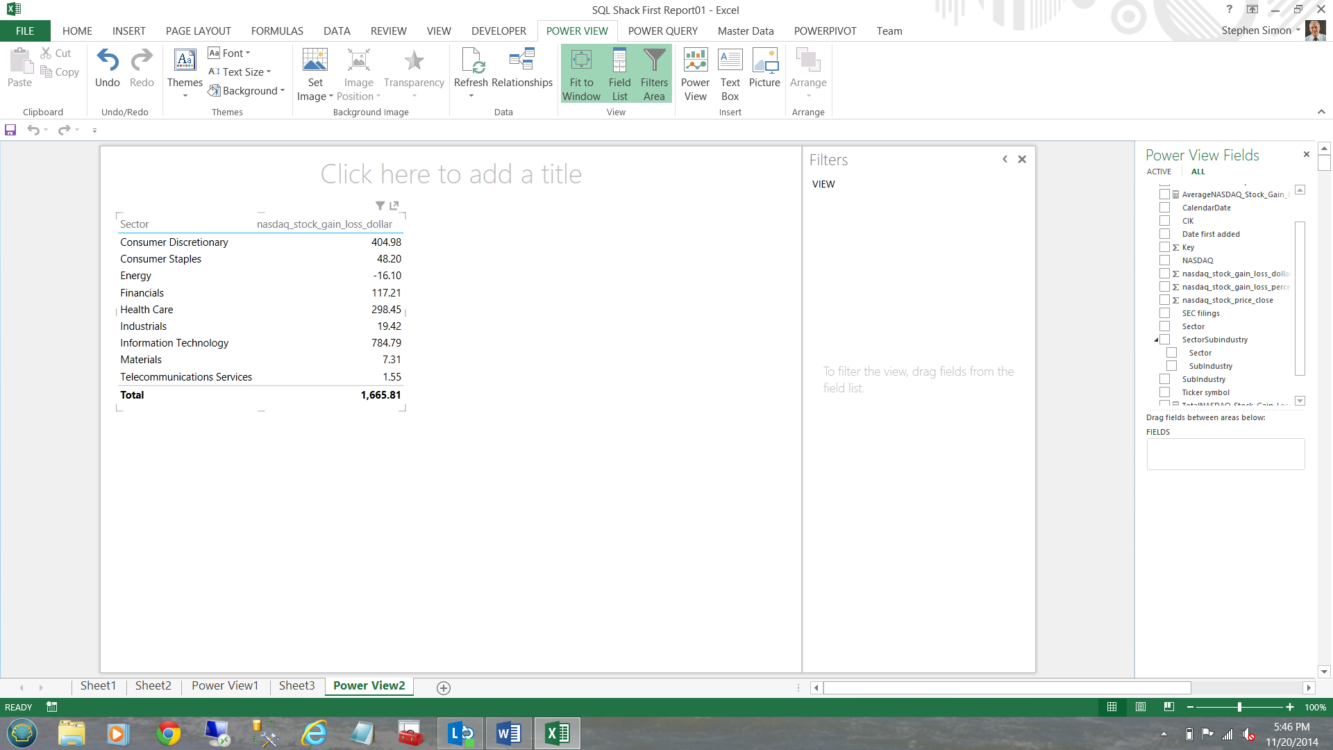
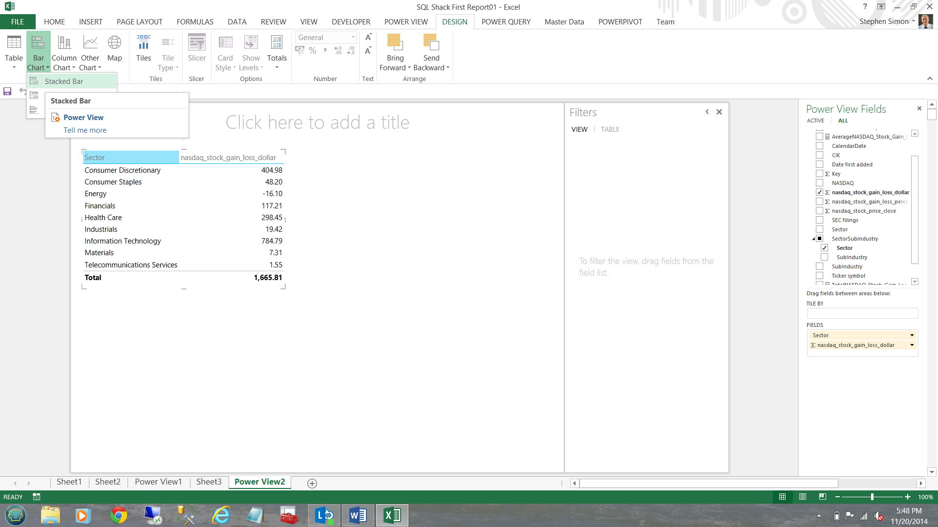
I now add the NASDAQ_STOCK_GAIN_LOSS_DOLLARS summary level totals (see below).
Now, I do not really like matrices thus I am going to convert the matrix to a chart.
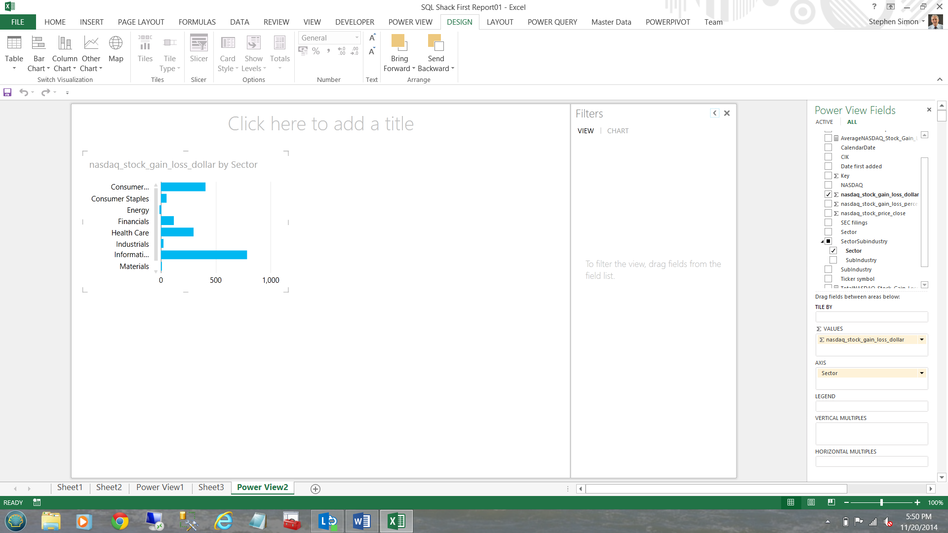
I click ‘Design’, ‘Bar Chart’ and Stacked (see below).
Our chart now appears.
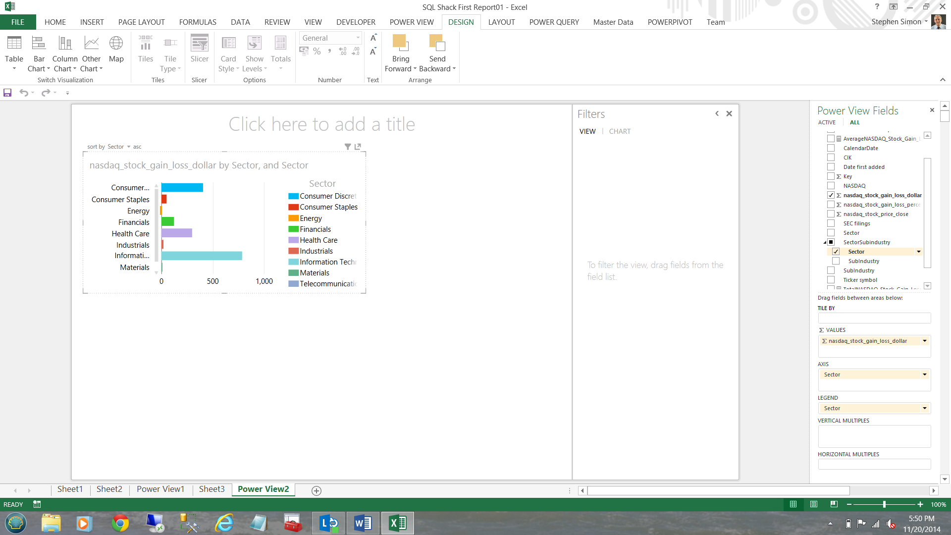
I drag the ‘Sector’ column to the ‘Legend’ box and the appearance of my chart changes (see below).
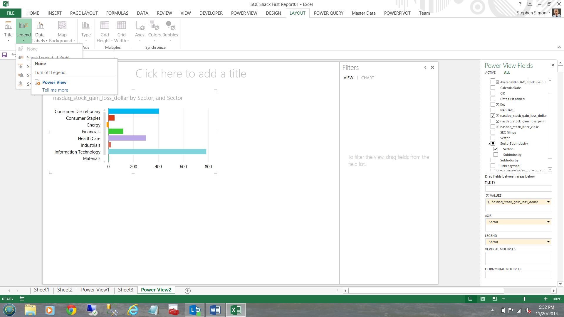
Clicking ‘Layout’ and ‘Legend’ and ‘None’ I am able to remove the legend box (to the right of the chart). The end result is that I now have more ‘real estate’ (see below).
Having completed this I go back to my fields on the right and now check mark the ‘SectorSubindustry’ hierarchy (see below and to the right of the screen shot).
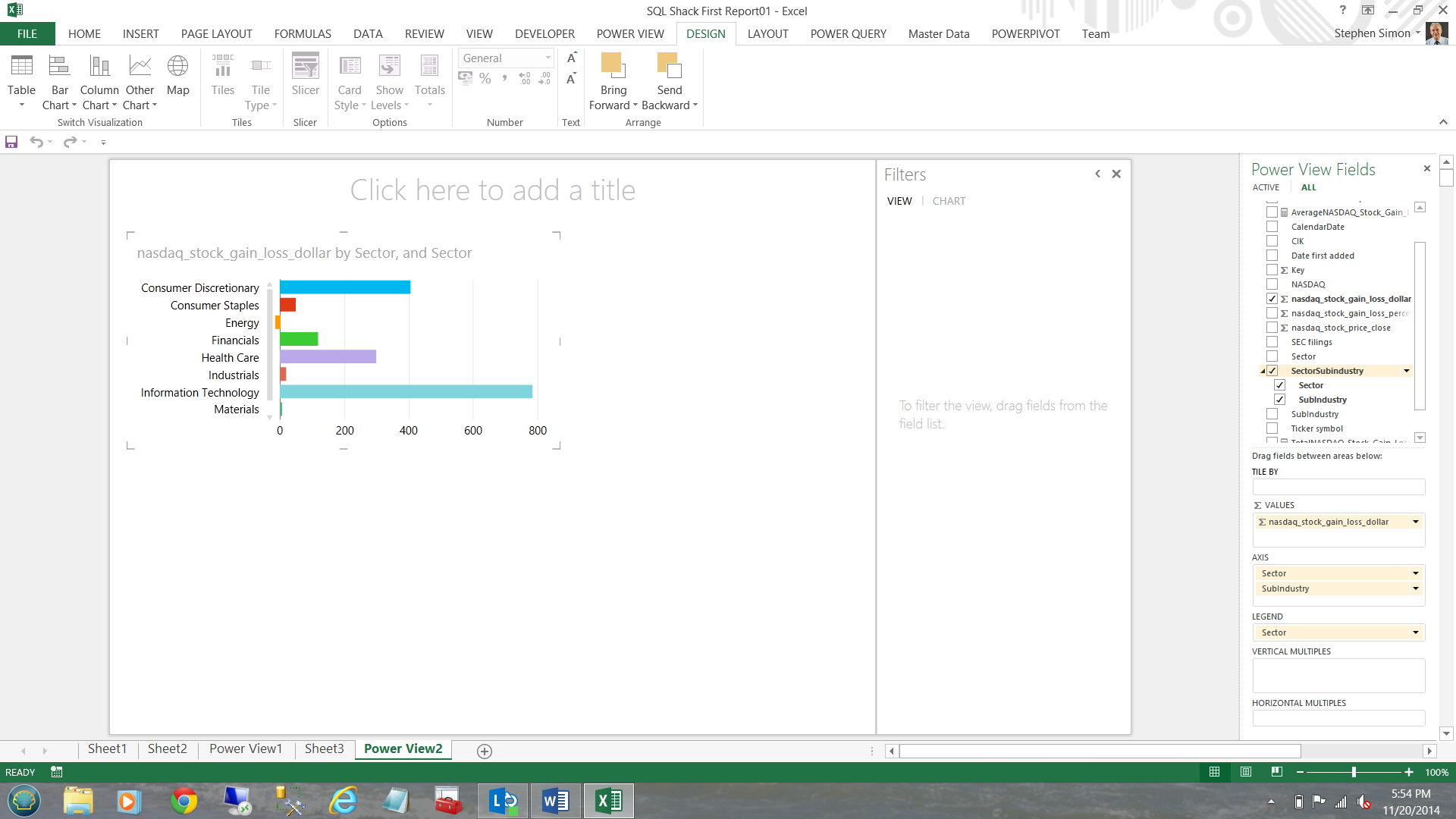
We have now completed our sector chart.
Wait a minute, what happens should I wish to see a particular sector broken down into sub-industries.
Double clicking on the ‘Information Technology’ sector (aquamarine) above enables us to drill through to the sub industries (see below).
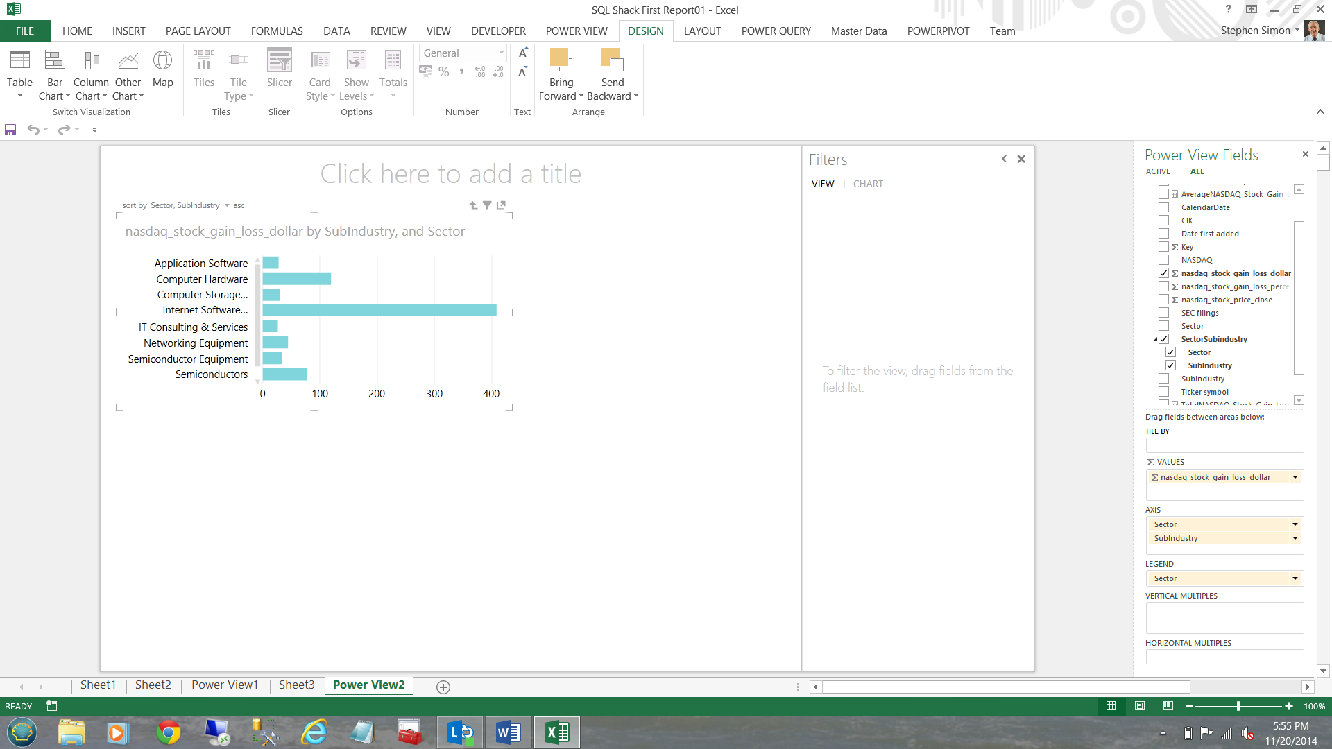
To return to the parent, one simply clicks the ‘up arrow’ immediately below the word ‘add’ in ‘Click here to add a title’
This completes our very first Power View Report.
Working with maps
Often users perform ‘what if scenarios’ including looking at the demographics of their current markets. The client mentioned above was no exception. We shall now look at a variation on the same map based theme that I created for this client.
To create a map based report, we shall create new query.
The query may be constructed in a new workbook or within the same workbook that we have been using thus far.
To start, I choose ‘PowerPivot’ and ‘Manage’.
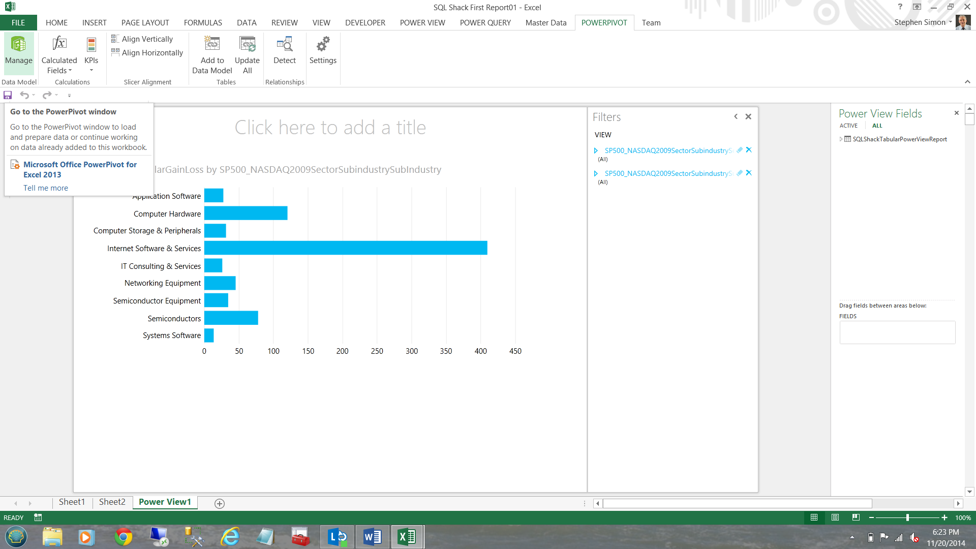
I choose an existing connection by selecting our ‘SQLShackTabularReportingModel’ (see below).
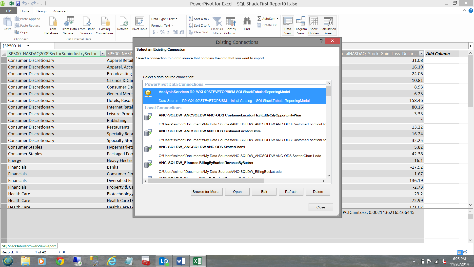
Clicking ‘Open’ our MDX query box opens. This is the same query box that we have seen above. Once again and as described above, I open the design box.
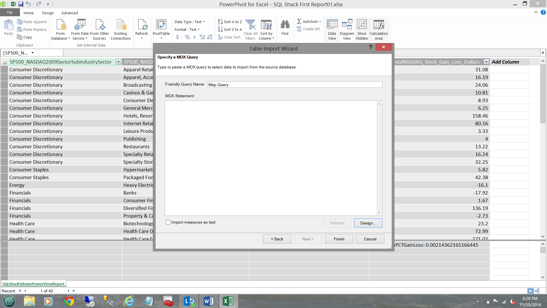
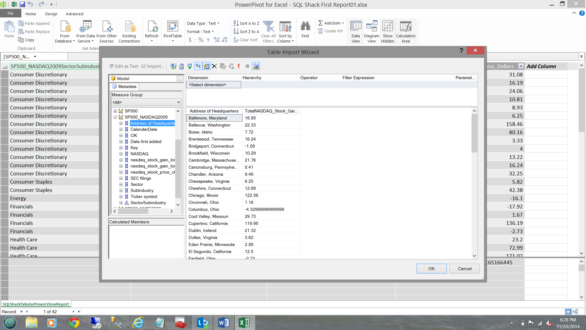
I drag ‘Address of Headquarters’ and ‘TotalNASDAQ_Stock_Gain_Loss_Dollars’ to the screen (see below).
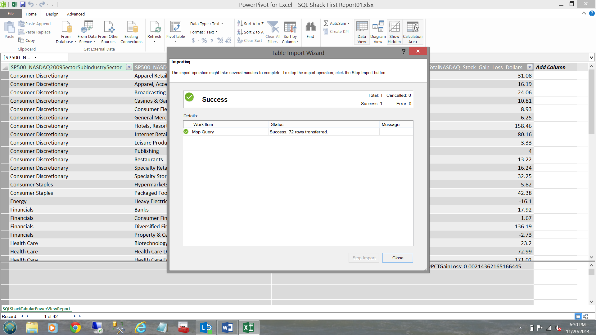
I complete the same process (as was previously discussed) by approving my selection and clicking ‘OK’. Once again I receive indications that all went well (see below).
I exit now exit from PowerPivot.
Creating our first map based report.
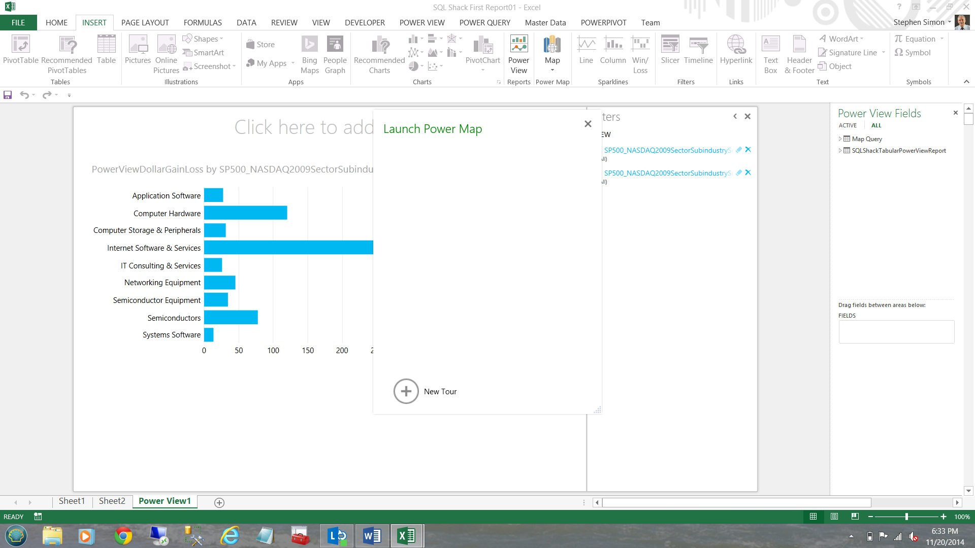
Selecting ‘Insert’ from the main menu and ‘Map’, I am able to launch Power Map.
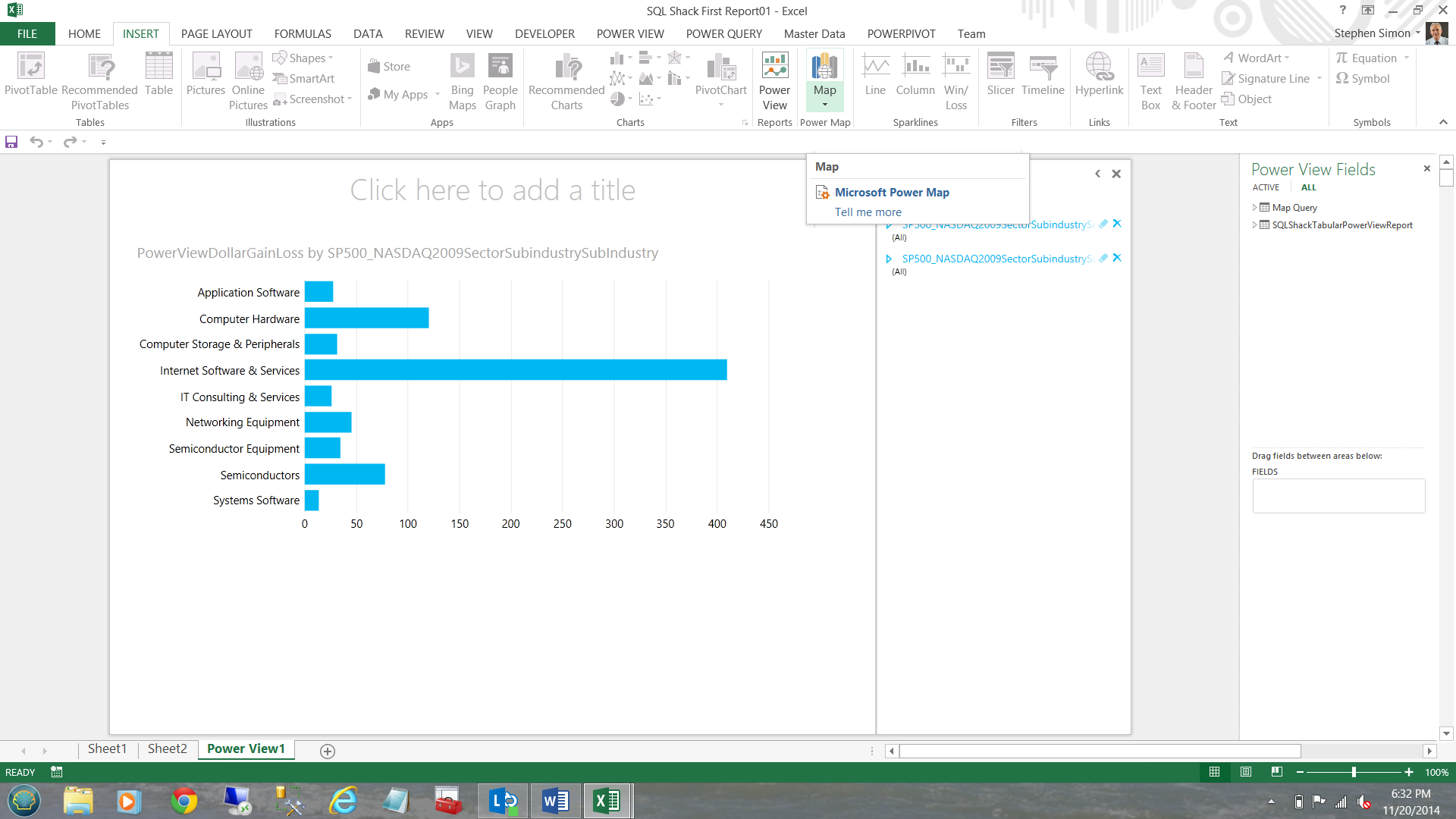
I click ‘New Tour’ (see below).
Power Map will now appear on your screen.
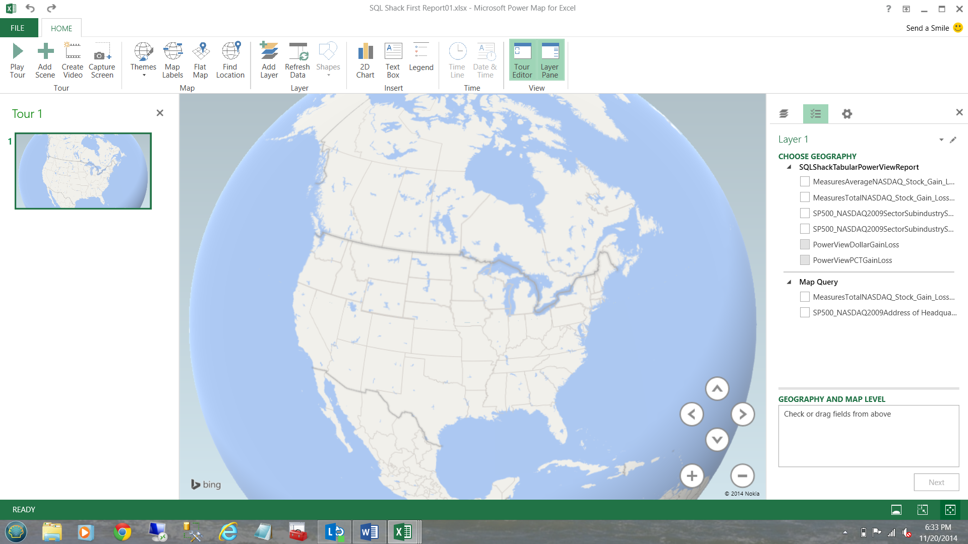
I drag the ‘SP500_NASDAQ2009Address of Headquarters’ into the ‘Geography and Map Level’ box (see below).
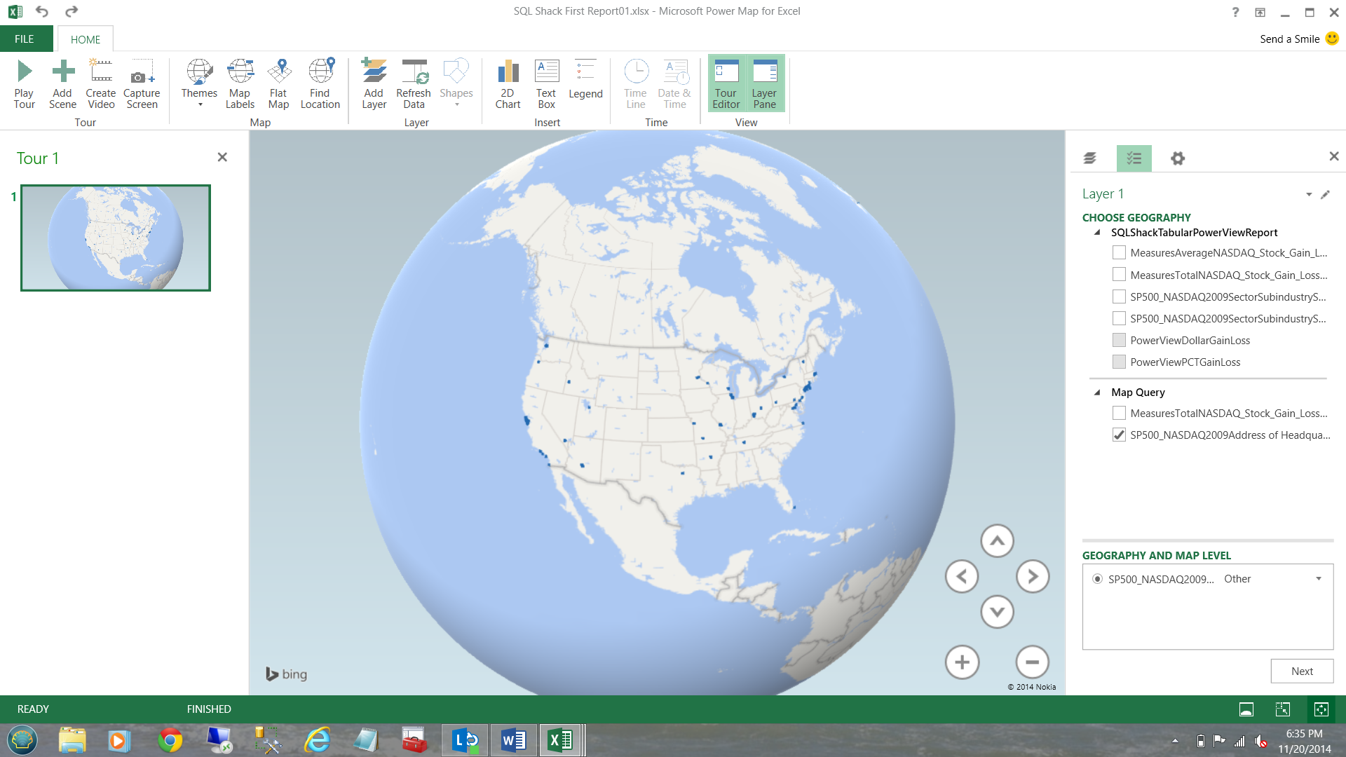
NOTE that the locations of the varied headquarters appear as blue dots on the map of the US.
Clicking next, I am able to add the financial figures.
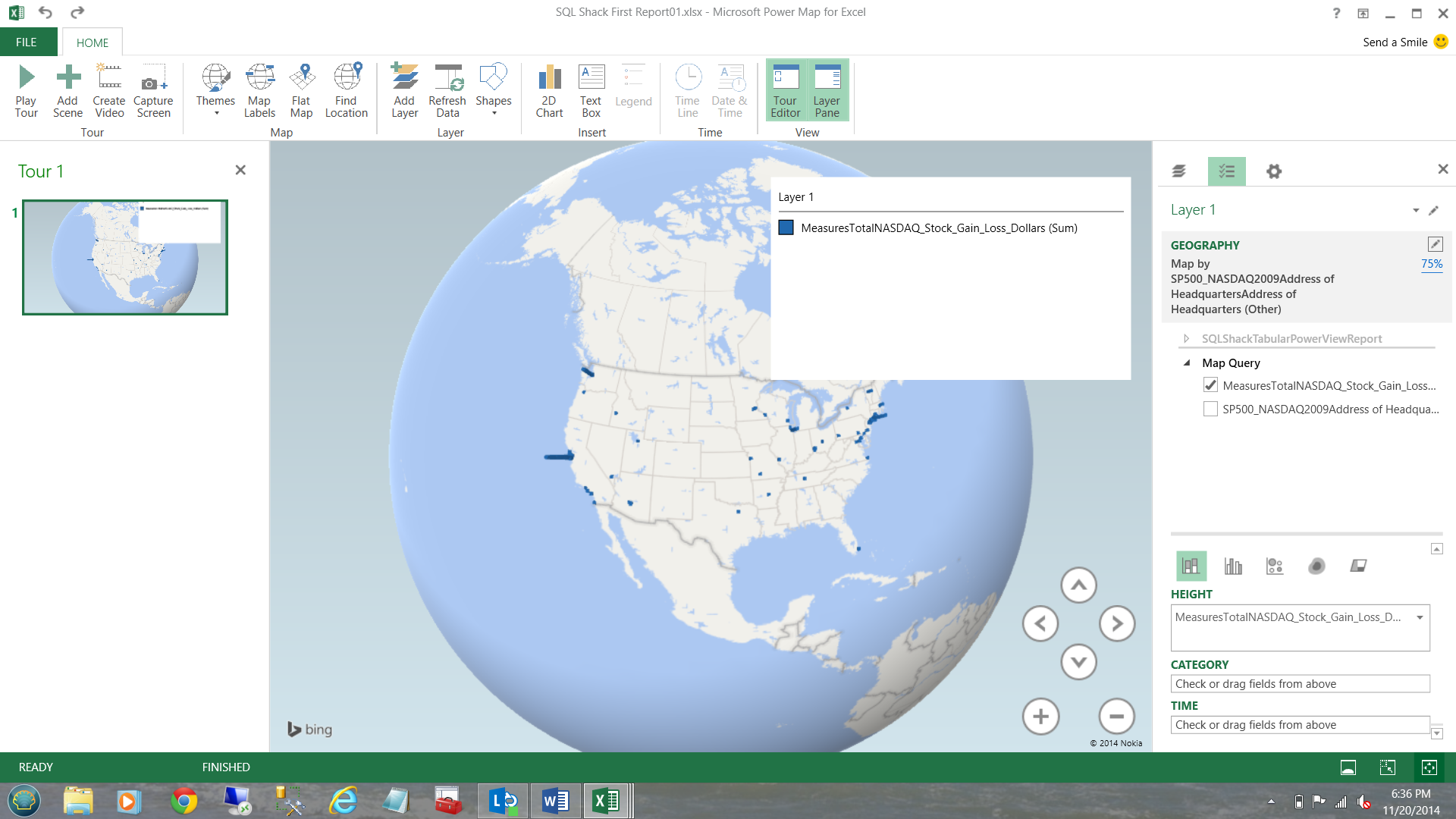
Once again, NOTE the way the value of the measures are shown on the map. If one zooms in, the relief is really cool. Oh yes!!! A ‘gotcha’: you must be connected to the internet for the Bing maps to be rendered.
This completes our quick venture into the world of Power BI.
Conclusions
Working with folks from the financial world presents challenges even at the best of times. From practical experience, these folks are more receptive to change when we can work within their comfort zone (a spreadsheet).
The new tabular model (BISM) introduced with SQL Server 2012 has the same look and feel as conventional spreadsheets, but provides much more flexibility including reporting capabilities to a plethora of front end GUI’s. These include Excel, SQL Server Reporting Service and reports hosted on SharePoint.
This completes our quick venture into the super world of Power BI. I certainly hope that I have raised more questions than answers.
Until the next time, happy programming!
Useful references
Getting started using solely Excel and Office 365
The links to the freely available source data that I have used above may be found on this site. As a caveat, should you try to work through the exercise beware many parts do not function as they should. Finally this exercise is NOT SQL Server based.
Steve has presented papers at 8 PASS Summits and one at PASS Europe 2009 and 2010. He has recently presented a Master Data Services presentation at the PASS Amsterdam Rally.
Steve has presented 5 papers at the Information Builders' Summits. He is a PASS regional mentor.
View all posts by Steve Simon
- Reporting in SQL Server – Using calculated Expressions within reports - December 19, 2016
- How to use Expressions within SQL Server Reporting Services to create efficient reports - December 9, 2016
- How to use SQL Server Data Quality Services to ensure the correct aggregation of data - November 9, 2016