

Introduction
Last month I ran two Business Intelligence pre-conferences in South Africa. A interesting request arose during the course of the preconference in Cape Town. The individual wanted an approach to extracting data from an OLAP cube that would avoid intensive utilization of MDX and more reliance upon T-SQL. His main concern was with filtering the data at run time, via the report front end.
In this “fire side chat” we shall do just that, utilizing the cube that comes with the new Microsoft database “WideWorldImporters” and we shall learn how we can get from this
|
1 2 3 4 5 6 7 8 9 |
SELECT NON EMPTY { [Measures].[Quantity - Sale], [Measures].[Unit Price - Sale], [Measures].[Ext Revenue], [Measures].[WWI Invoice ID] } ON COLUMNS , NON EMPTY { ([Customer].[Customer].[Customer].ALLMEMBERS * [City].[City].[City].ALLMEMBERS * [Invoice Date].[Date].[Date].ALLMEMBERS * [City].[State Province].[State Province].ALLMEMBERS ) } DIMENSION PROPERTIES MEMBER_CAPTION, MEMBER_UNIQUE_NAME ON ROWS FROM [Wide World Importers DW] CELL PROPERTIES VALUE, BACK_COLOR, FORE_COLOR, FORMATTED_VALUE, FORMAT_STRING, FONT_NAME, FONT_SIZE, FONT_FLAGS |
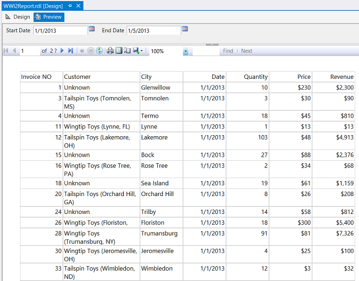
to this!
Preparitory work
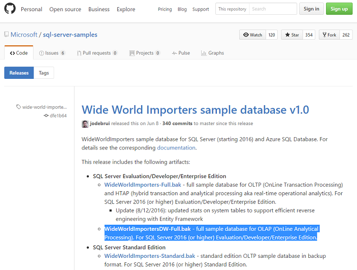
Should you not have a copy of the WideWorldImportersDW, please do download a copy of the relational database. The relational database may be found at this link
Simply restore the database to your desired SQL Server 2016 instance.
We are now ready to begin.
Getting started
Opening Visual Studio 2015 or the latest version of SQL Server Data Tools for SQL Server 2016, we create a new Analysis Services project as shown below.
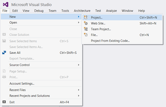
Opening Visual Studio of SQL Server Data Tools, we select “New” and “Project” (see above).
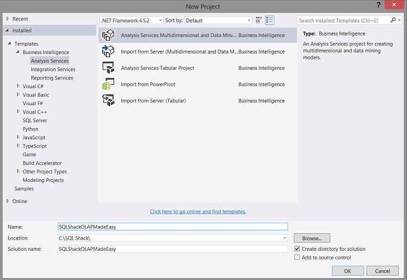
We give our project a name and select the “Analysis Services Multidimensional and Data Mining…” option (as shown above). We click “OK”.
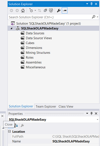
Our design surface is brought into view (see above).
Our first task is to add a data source. We right click upon the “Data Sources” folder shown above.
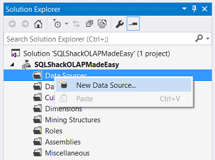
We select “New Data Source” (see the screenshot above).
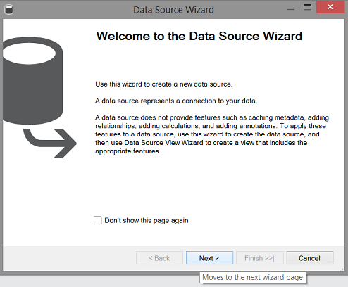
The “Data Source Wizard” is brought into view. We click “Next” (see above).
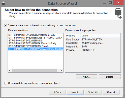
We are presented with a list of existing data connections. The “eagle eyed” reader with note that a connection to the relational database already exists however we shall create a NEW connection for those of us whom are not that familiar with creating NEW connections.
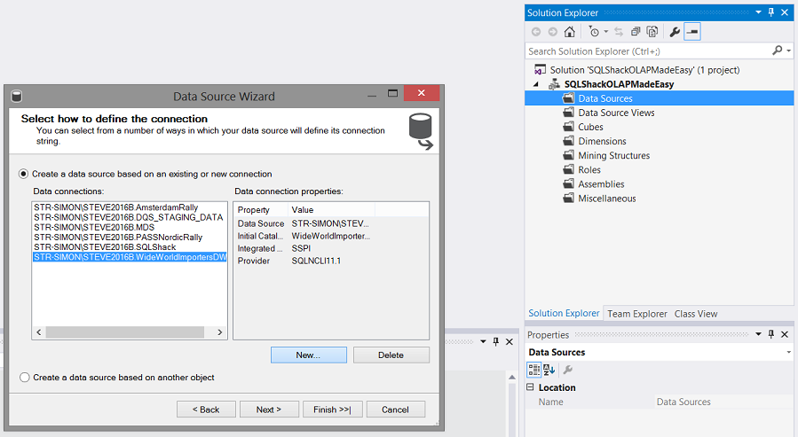
We click the ”New” button as may be seen above.
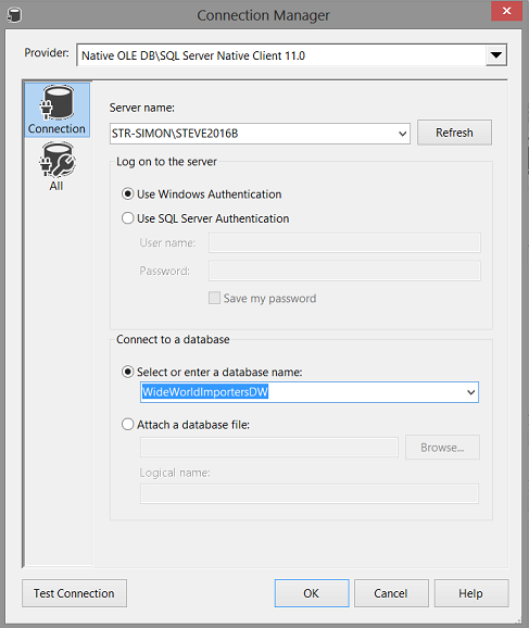
The “Connection Manager” wizard appears. We set our server instance name and select the “WideWorldImportersDW” relational database (as may be seen above). We then test the connection and we click “OK” to exit the wizard.
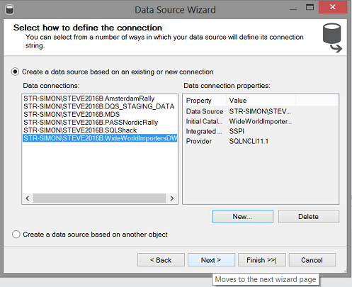
We find ourselves back upon back within the “Data Source Wizard”. We select our new connection and click “Next” to continue.
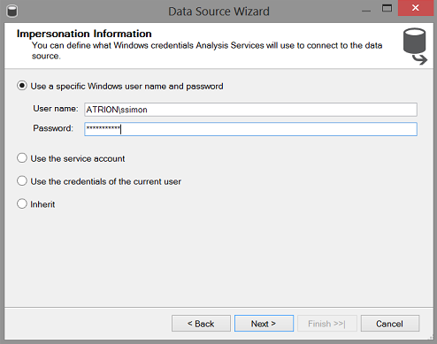
The reader will note that we are now request to enter our “Impersonation Information”. In this instance I have opted to utilize a specific user name and password. This data will be used to validate that we have to necessary rights to publish our project to the Analysis Server.
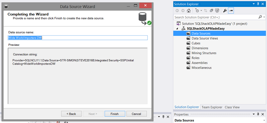
Finally, we give our data source a name and click “Finish” to complete the process (see above).
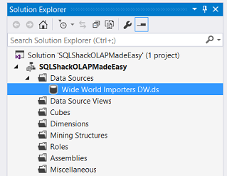
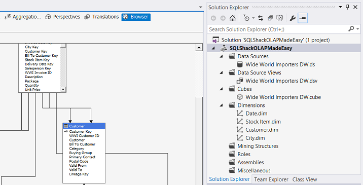
The data source that we have just created may now be seen under the “Data Sources” folder as shown above.
Creating the “Data Source View”
Our next task is to create a “Data Source View”. Whilst we have created a data connection, all that the connection does is to permit our project access to the relational database. Now we must tell our project, which data we want to view and this is achieved through the “Data Source View”.
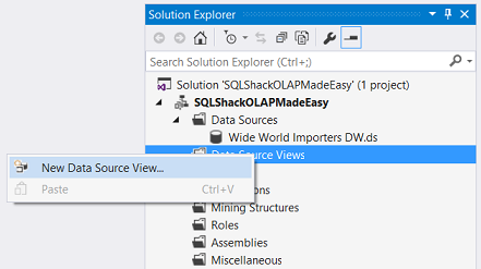
We right click upon the “Data Sources Views” folder and select “New Data Source View” (as may be seen above).
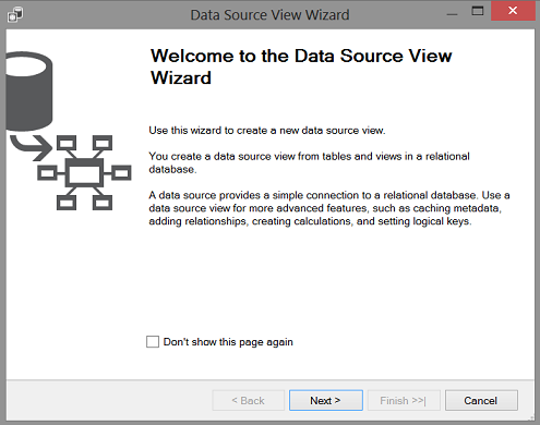
The “Data Source View Wizard” is brought into view. We click “Next”.
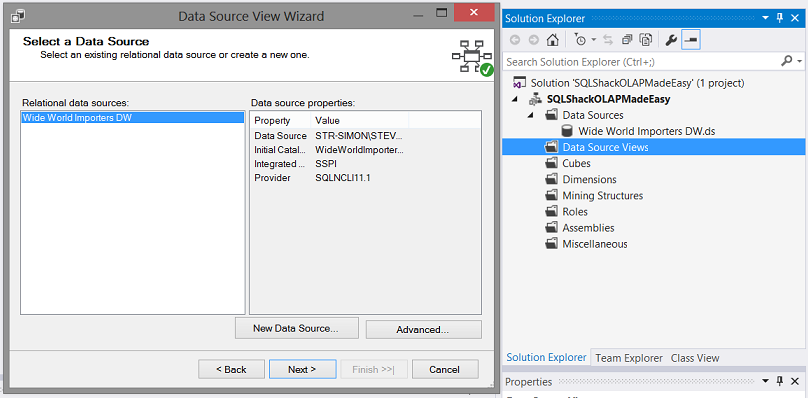
The wizard now shows us our “Wide World Importers DW” data connection that we created above. We select this connection and click “Next”.
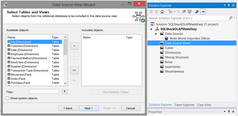
A list of table now appears. We select the tables that we wish to work with, as may be seen below:
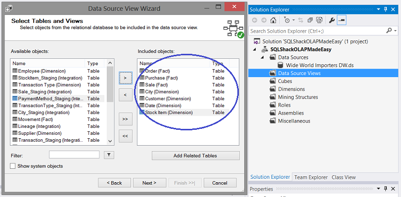
Viewing the “Included objects” dialog box we note the tables that we shall include within our view. All the table “inter-relationships” (e.g. keys and foreign keys) will be respected and this is why we must ensure that all the necessary tables are included in the model that we are creating. Failure to do so, will result in issues within the cube.
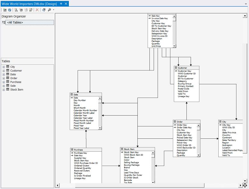
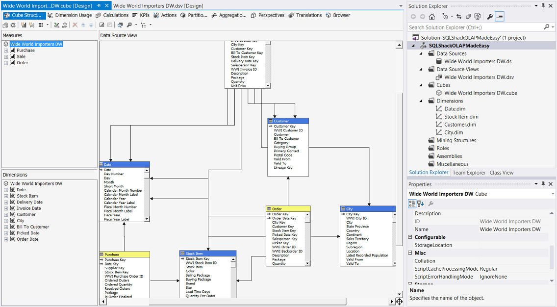
Upon completion of the “Data Source View” we are returned to our drawing surface and our completed “relationship diagram” appears (see above).
Creating our cube
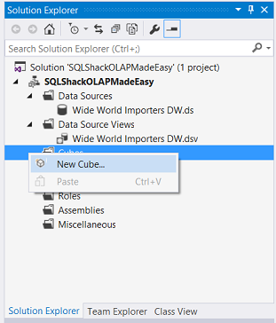
In order to create our desired cube, we right click on the “Cubes” folder and select “New Cube” (see below).
The “Cube Wizard” appears.
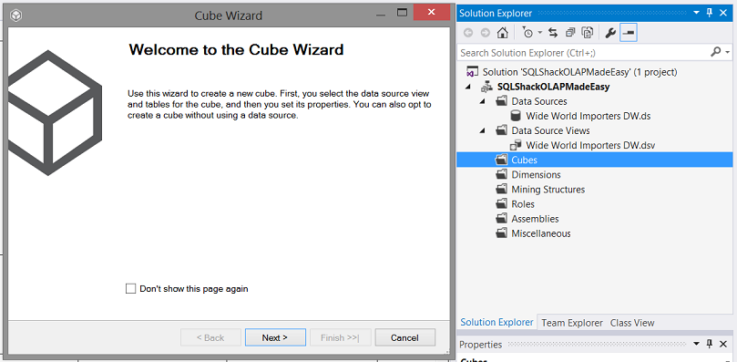
We click “Next” (see above).
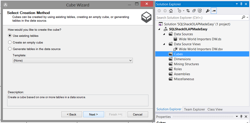
We opt to “Use existing tables” (see above). We now click “Next”.
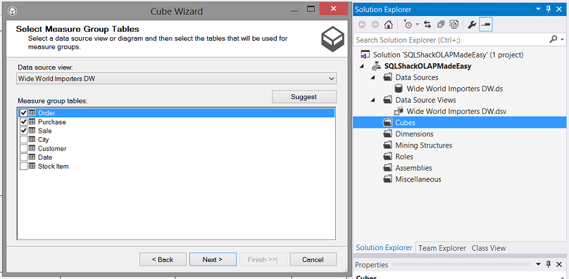
We are requested to select our “Fact / Measures” tables. These are the tables that contain data such as the monitary values of purchases / sales / orders. These tables are the quantifiable tables.
We select Order, Purchase and Sale (see above). We then click next.
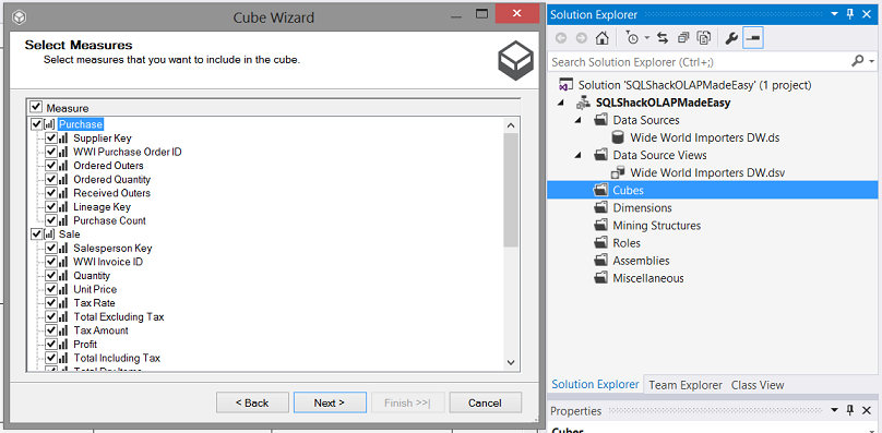
We are now presented with the “attributes” (of these fact tables) that will be included within the cube. We have the option to remove any unwanted attributes however for our present exercise, we shall accept all the attributes. We click “Next”.
Selecting our dimensions or “qualitative attributes”
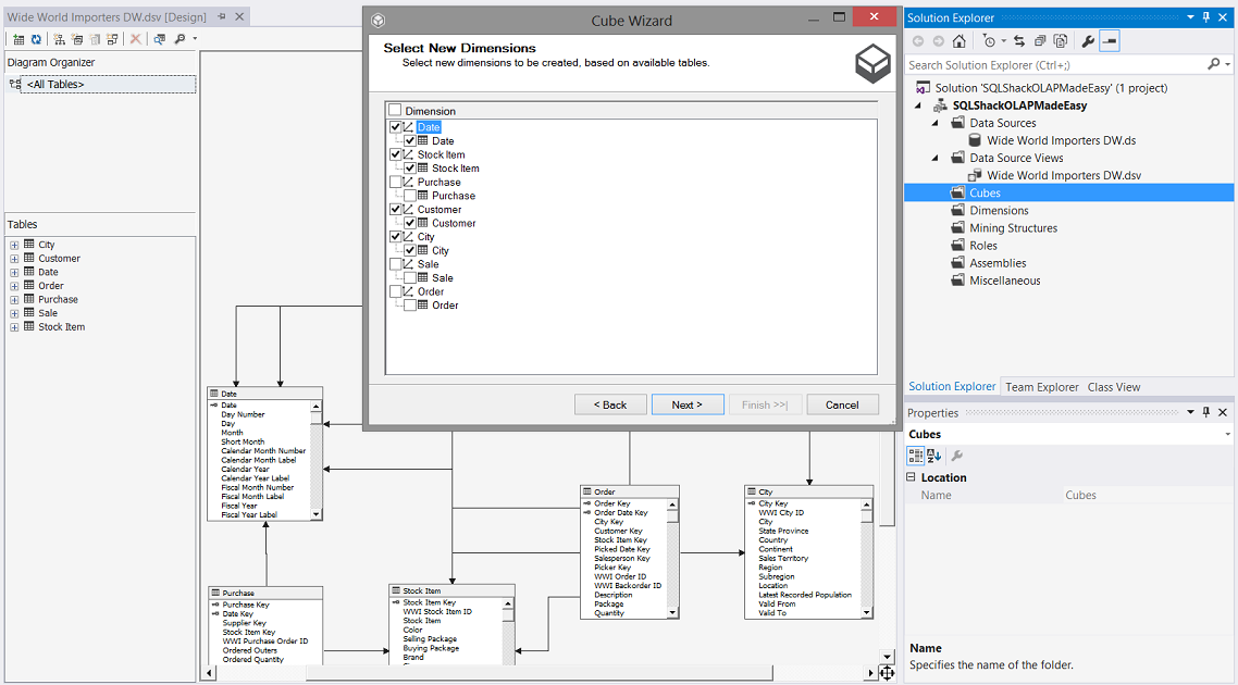
We are now asked to select our “Dimensions” (see above). We select “Date”, “Stock Item”, “Customer” and “City” (see above). We click “Next”.
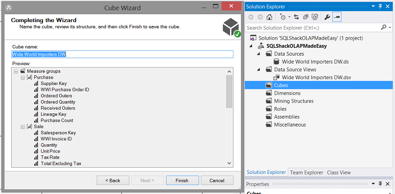
The fields within the Dimensions are shown to us and we click “Finish”.
Customizing our Dimensions
Prior to continuing we have one further task to perform on our dimensions. Whilst the dimensions themselves exist, not all the necessary ATTRIBUTES are present within the “dimension” itself (see below).
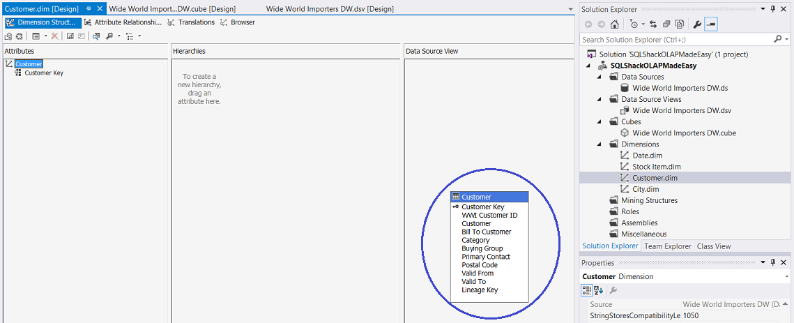
Double clicking upon the “Customer” dimension (see above), we open the attribute editor. We note that only the key is shown. We require more attributes and these attributes are located within the Customer table shown above.
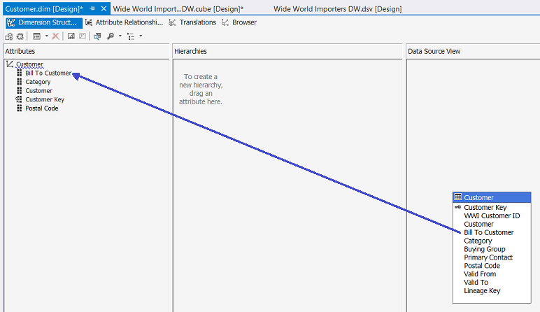
We drag “Bill to Name”, “Category”, “Customer” and “Postal Code” to the Attributes box from the bottom right list of Customer attributes (see above).
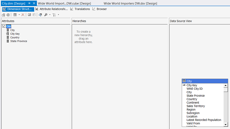
We do the same for the “City” attributes as may be seen above.
We now are in a position to process our cube and extract information from the Cube.
Processing our cube
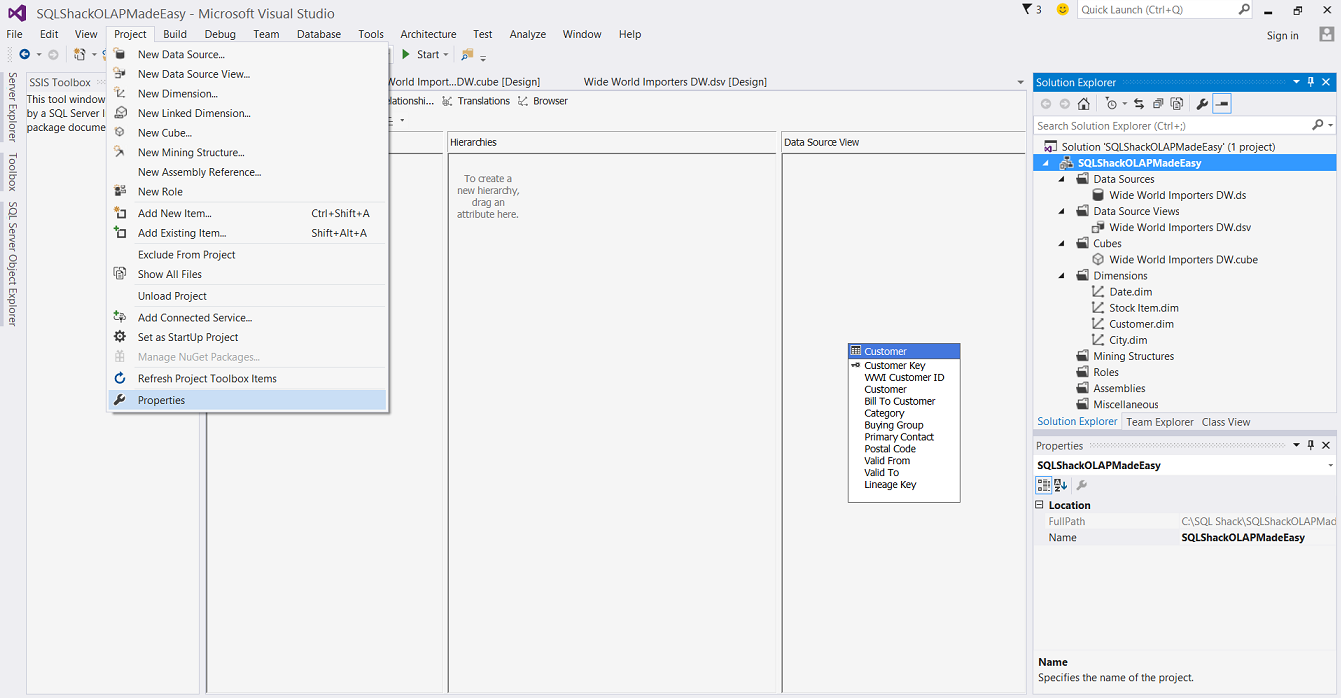
Clicking on the “Project” tab, we select the “Properties” (see above) .
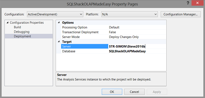
We must now tell the system to where we wish to deploy our project, as well as to give the target OLAP database a name (see above). We click “OK” to leave the “Properties Page”.
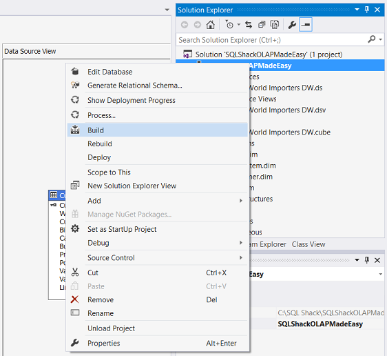
We shall now “Build” or attempt to “Compile” our solution to detect any errors.
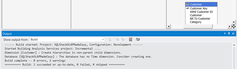
The “Build” succeeds.
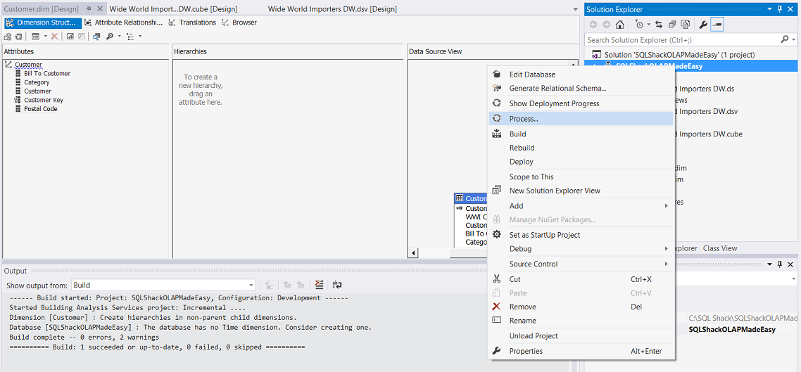
Once again, we right click upon our Project name (see above) and we select “Process” from the context menu (see above).
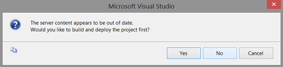
We are informed that the “Server content appears to be out of date”. We tell the system that we want to build and deploy the project.
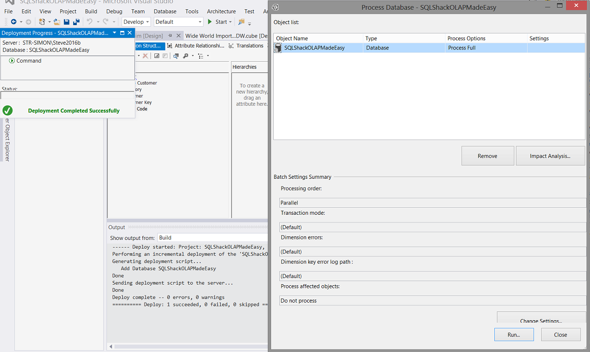
We are informed that the deployment was successful (see above in green) . The “Process Database” dialogue box appears asking us if we wish to process the database. We click “Run”.
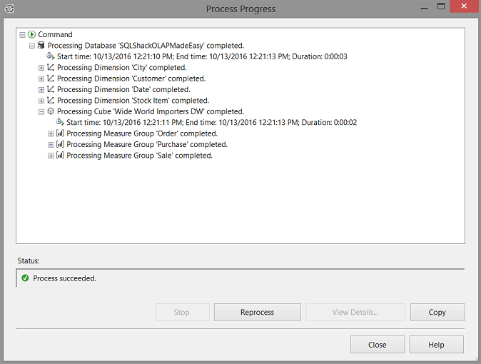
Upon completion of the processing and if no errors were encountered, we are informed of “Successful processing” (see above). What this “processing” achieved was to create aggregated financial results for all customers, for all cities within the realm of the given data. We close all open processing windows.
We now find ourselves back within the Cube designer surface. Let us see what kind of results we can observe.
Clicking upon the “Brower” tab, brings up the “Cube Browser” (see above)
Prior to creating our first MDX query, we decide that we wish to create a calculated field for “Revenue”.
Revenue is defined as the quantity sold * unit price. We click upon the “Calculations” tab and create a new “Calculation”.
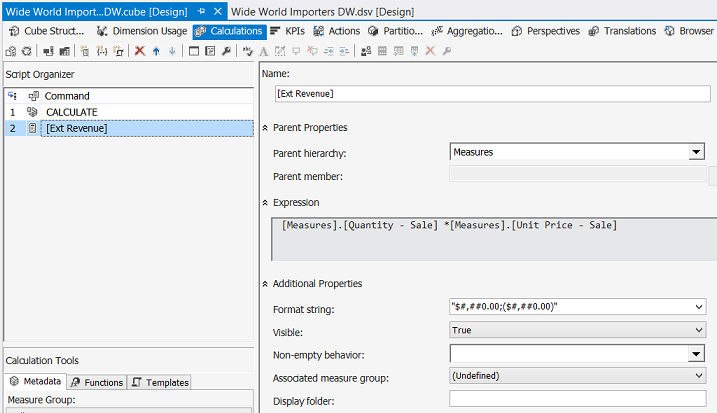
Our new calculated field may be seen above and it is defined as “Quantity – Sale” * “Unit Price – Sale”.
With our calculated field being designed, we are now in a position to browse our cube. We reprocess the cube and then click upon our Broswer tab (see above) .
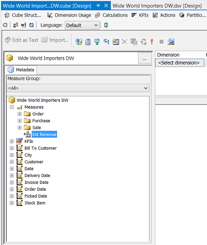
We note that our calculated field appears below the measure tables. This is normal and the calculation is ready for us to utilize.
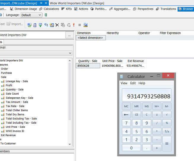
We drag “Quantity- Sale” , “Unit Price – Sale” and our calculated field “Ext Revenue” onto the design surface. The reader will note that the aggregated values of all the data are shown in the one row above. Further using a calculator and mulitplying the figure together, we confirm that our calculated field is working accurately. The only issue being that the one aggregated row is of little use.
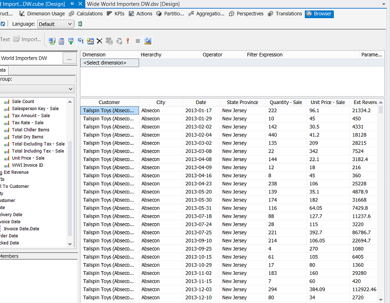
By adding the “Customer Name”, the “City” ,the “Invoice Date”, Invoice No” and the “State Province” we see the revenue from each invoice for each invoice date. In short we have more meaningful results.
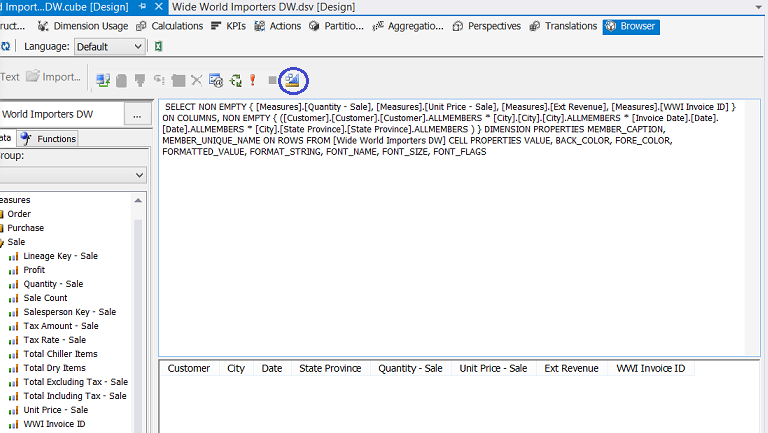
By clicking on the “Design Mode” tab we see that MDX code behind the data extract that we created above. This code becomes important as we shall use this code for the report query that we shall create in a few minutes.
As a double check that we are in fact on the right footing, we now call up SQL Server Management Studio and login to our OLAP server. We select the SQLShack OLAP database that we just created.
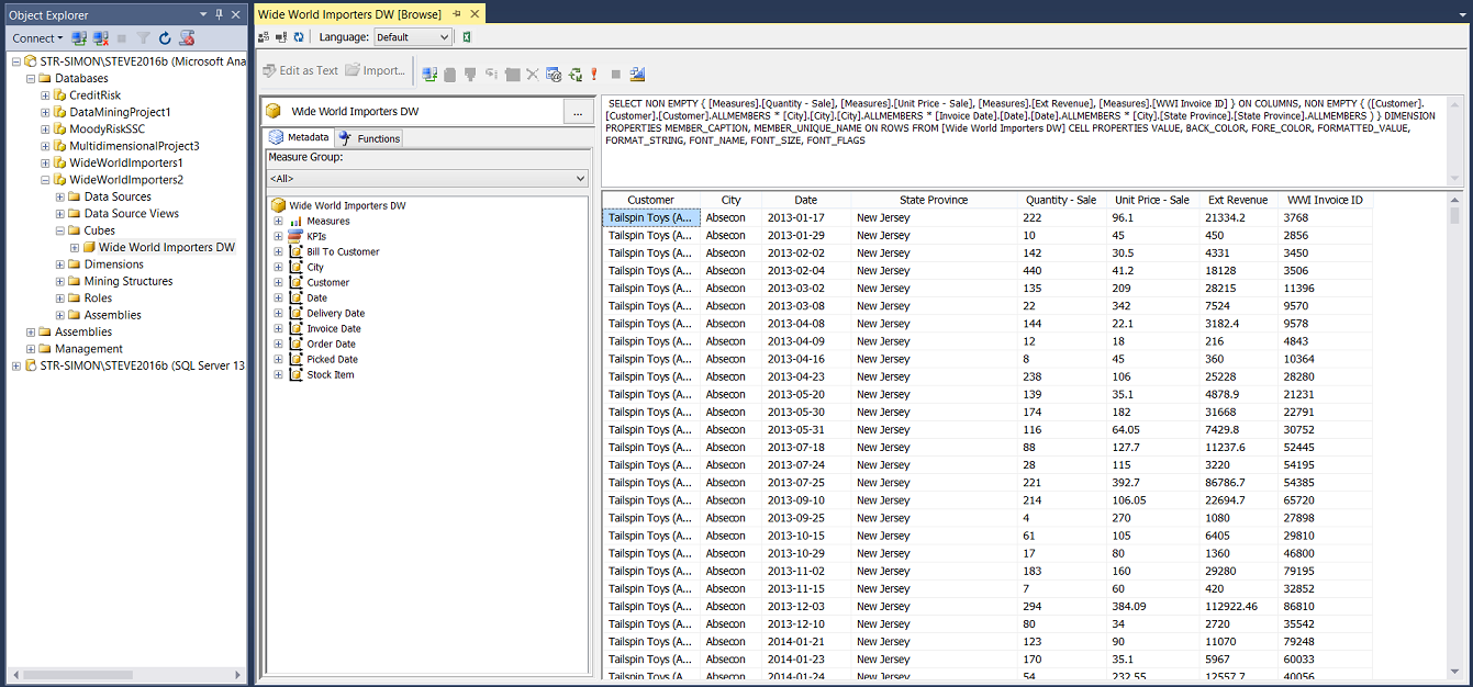
Utilizing the MDX code from our Visual Studio project we can copy and paste the same code into the Cube Browser within SQL Server Management Studio. The results may be seen above.
The “Wild Card”
Before proceeding to create our reports, we have one final task to perform. We are going to create a linked server to our Analysis database that we have just constructed.
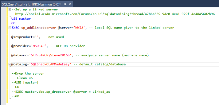
This is the code that we shall utilize and the code itself may be found in Addenda 2.
Now that our linked server has been created, we are in a position to begin with our report query!
Creating our report query
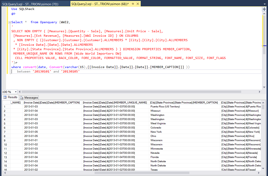
Opening SQL Server Management Studio, we open a new query. Utilizing the DMX code that we obtained, we place that code within an “OpenQuery” utilizing our new linked server (see below).
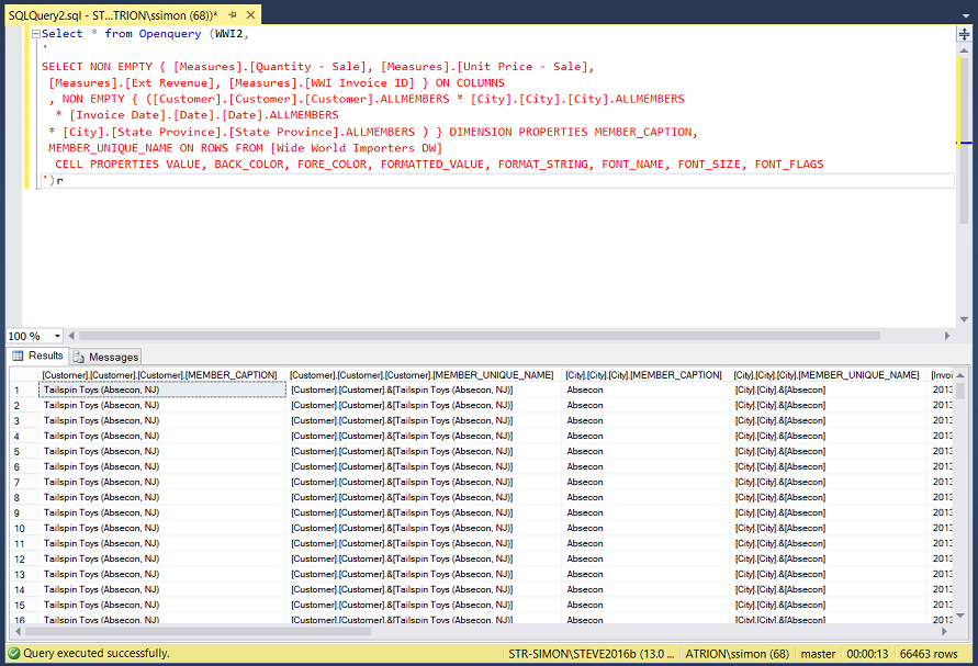
Now, the “wise acre” will question, why are we doing this. The answer is fairly simple. The sub query is the MDX query and the outer query is developed in T-SQL! Being developed in T-SQL permits us to filter the result set utilizing all the “goodies” such as case logic within the T-SQL portion predicate. Yes, we are pulling all the AGGREGATED data from the cube however if the data is properly aggregated during the processing of the cube , then the “hit” is not that bad.
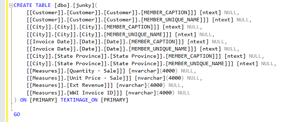
The one point that is not immediately obvious is that the true names of the extracted fields are not what one would expect. Normally and as a once off we publish the results of the query to a table. This will enable us to determine the correct names of the fields as seen by SQL Server (see below).
Modifying the query slightly we can now add a T-SQL date predicate (see below):
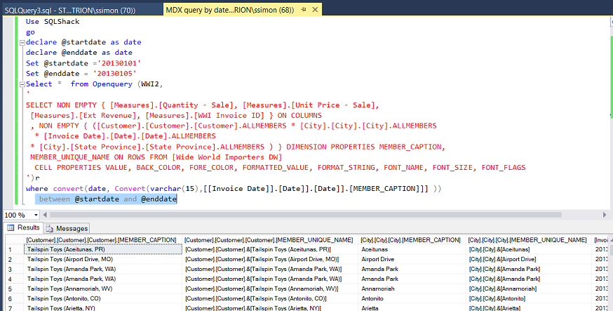
The reader will note that the start and end dates have been hard wired. We are going to alter this so that the predicate accepts a start and end date from parameters (see below):
Our last modification to our query is to create a stored procedure, which will be utilized by our report.
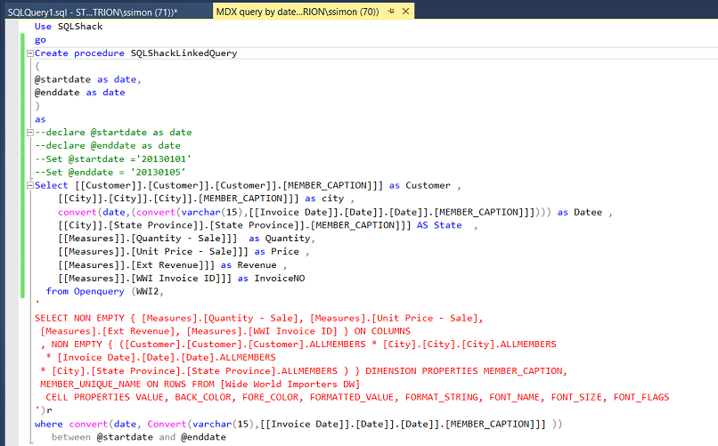
The reader will note that we have selected a subset of the fields necessary for our report. As a reminder the field names appear a bit wonky however this is the way that SQL Server “sees“ them.
Creating our report
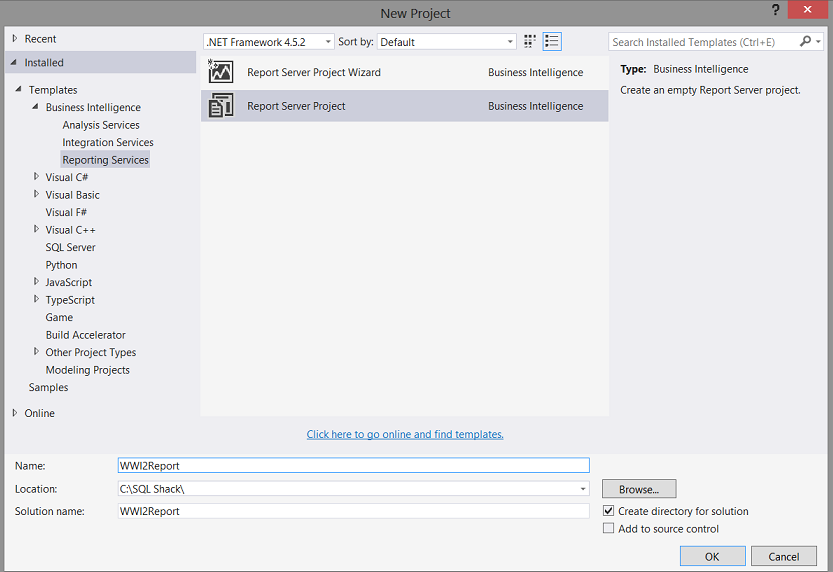
Once again we open Visual Studio 2015 or SQL Server Data Tools version 2010 or above. This time however we choose a “Report Services Project” (see above). We give our project an name and click “OK” (see above).
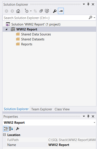
Having created the project we are now brought to our design surface. Our next task is to create a new “Shared Data Source” which will connect to our relational database table. As we have discussed in past “get togethers”, the database may be likened to the water faucet on the side of your house. The “data source” may then be likened to a water hose that will carry the data to where it is required.
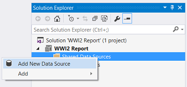
We right click on the “Shared Data Sources” folder (as above). We select “Add New Data Source”.
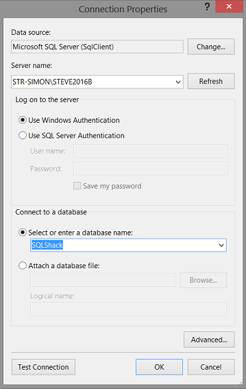
The “Connection Properties” dialogue box opens. We tell the system the name of the SQL Server Instance and database to which we wish to connect (see above).
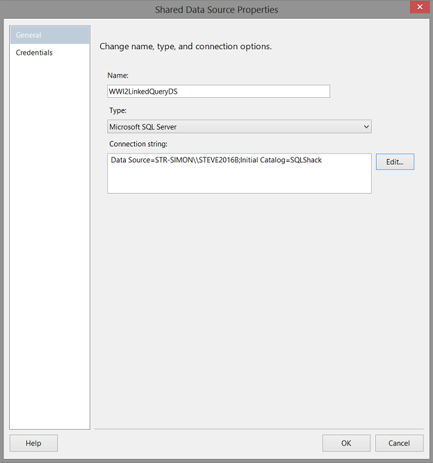
We are returned to the “Shared Data Source Properties” dialogue box (as may be seen above). We click “OK” to continue.
Configuring our new report
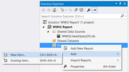
Our next task is to create our report. To do so we right click upon the “Reports” folder and select “Add” and then “New Item”.
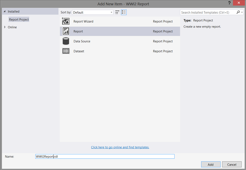
We find ourselves on the “Add New Item” screen. We select “Report” and give our report a name (as shown above). We click “Add” to continue.
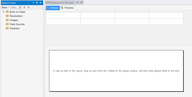
We find ourselves on our report design surface.
Now that we are on the report design surface, our first task is to define two parameters that may be utilized to pass a start and end date to our report query. The reader is reminded that when we created the initial query that we extracted records for a certain time frame. This time frame will be determined by the arguments passed to the query via the two parameters.
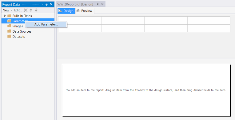
We right click upon the “Parameters” folder and select “Add Parameter” (see above).
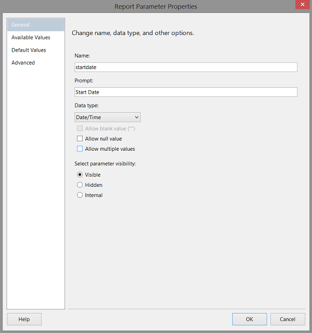
We assign a name to our parameter and set the data type to “Date / Time” (see above).
In a similar fashion we create and initialize our End Date parameter.
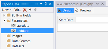
Our drawing “canvas” now appears as follows(see above).
Creating our Local Dataset
Now that we have created our parameters, we have one last structural task to complete and that is to create a dataset.
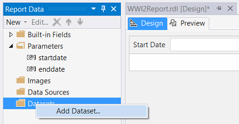
To create this dataset (which may be compared to a watering can which contains a “subset” of the water from the faucet on the house) , we right click on the “Dataset” folder and select “Add dataset”. As with the water can example, our dataset will contain the data that is extracted from our OLAP database via our query AND our linked server.
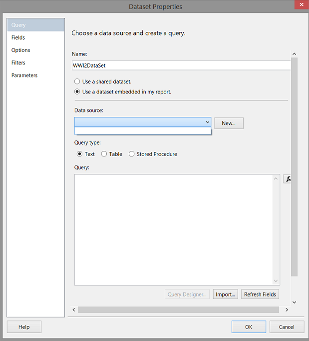
The “Dataset Properties” dialogue box opens. We give our dataset a name and as our dataset is a “local” dataset, we are required to create a new local data source that will be connected to the “Shared data source” that we just created. We click the “New” button (see above).
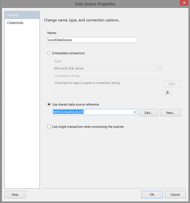
Having clicked the “New” button, we find ourselves on the “Data Sources Properties” dialogue screen. We give our local datasource a name and link it to our “Shared Data Source” (see above). We click “OK” to continue. We are returned to the ‘DataSet Properties” screen (see below).
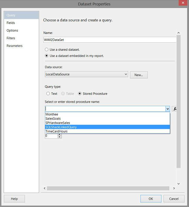
We select “Stored Procedure” for the “Query type” and using the drop down box, we select the stored procedure that we created above (see above).
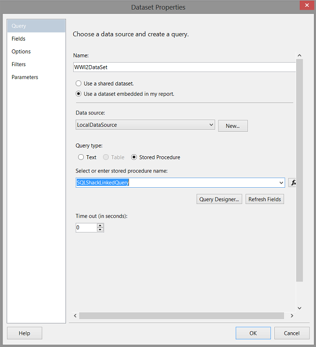
Having selected our stored procedure, we click the “Refresh Fields” button to bring in the list of fields that will be available to our report (see above).
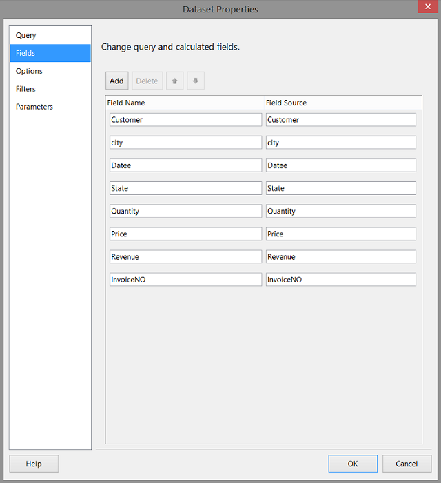
By clicking upon the “Fields” tab (upper left of the screen shot above) we may now see the fields that will become available to our report.
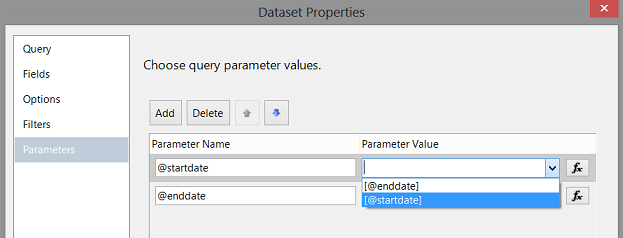
Clicking on the “Parameters” tab we note that the two parameters that we created with our stored procedure are now visible. These are the “Parameter Name” . The “Parameter Value” will come from user input (as arguments) via the two report parameters that we just created. Hence, we must assign the correct arguments to the stored procedure parameters.
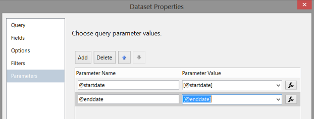
The screen shot above shows us the correct configuration.
Adding our report controls
Now that we have our report infrastucture or “plumbing” established, we are in a position to add the necessary controls required to allow the end user to view his or her data.
`
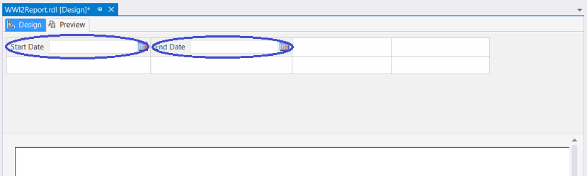
Our design surface shown above,the astute reader will note the two calendar controls (parameters) that we have just created.
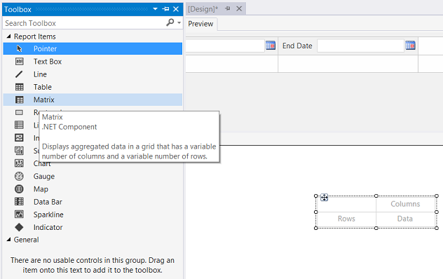
We drag a”Matrix” control from the tool box onto the drawing surface (see above).
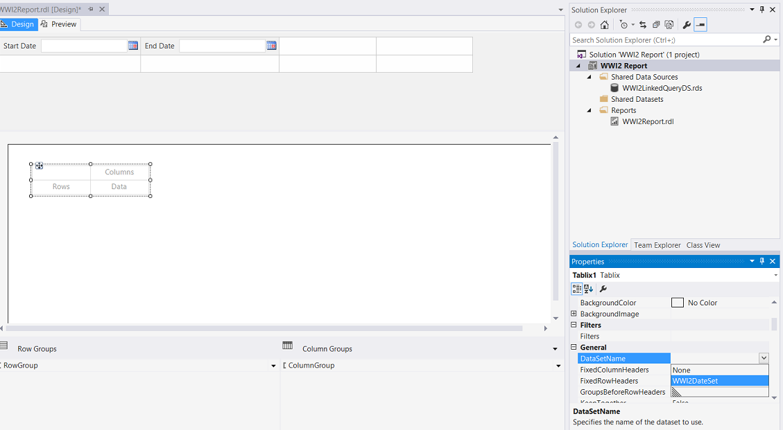
We click F4 to bring up the properties box of the matrix that we have just added to our work surface. We set its “DataSetName” property to the name of the dataset that we created above (see above).
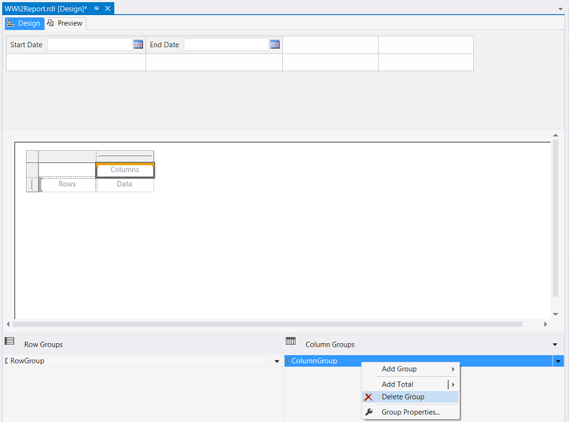
As we shall not be utilizing “Column Grouping”, we decide to remove the column grouping by right clicking upon the “ColumnGroup” and selecting “Delete Group” (see above).
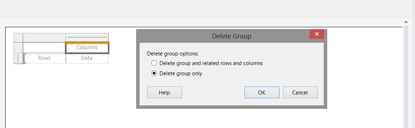
We are asked if we wish to delete the group and its related rows and columns OR merely to delete the grouping itself. We select “Delete group only” (see above).
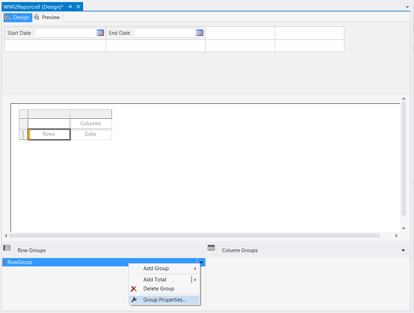
We do however wish to set the “Row Grouping” as we shall want to view our data as a summation of revenue by invoice number. We click upon the “Group Properties” tab.
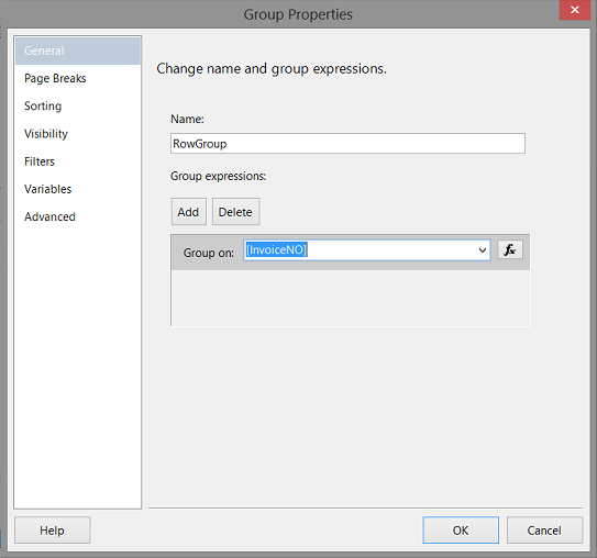
In the screen shot above, we set the grouping to be based upon invoice number.
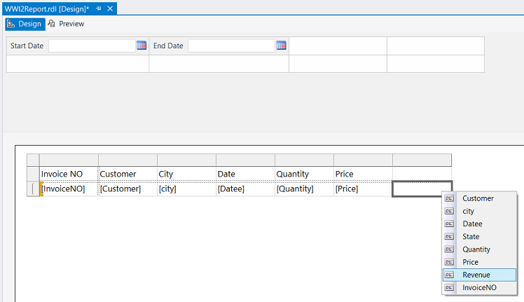
Our next task is to add the fields from the stored procedure to our matrix. This is shown above. We have discussed this process in detail in numerous past “chats”.
Our report construction is now complete.
Let us give it a whirl
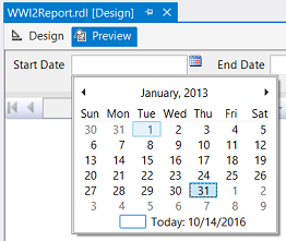
Clicking the “Preview” tab, we select the “Calendar” control and set the start date to 1/1/2013 (see above).
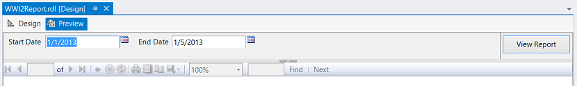
In a smilar fashion we set the end date to 1/5/2013 (see above). We now click “View Report”.
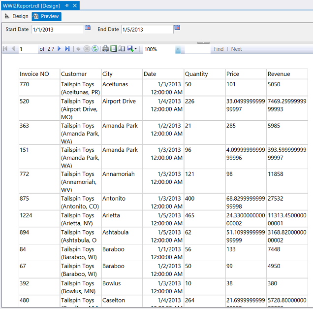
We note that our data is now visible to the user and that our report is now complete. Naturally the reader will want to sort and format the data. We have covered this as well in numerous past “get togethers” however the screen dump below shows our data sorted by invoice number and the numeric values have been rounded to the nearest dollar (see below).
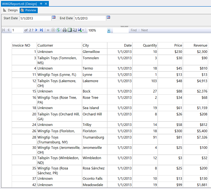
In order to polish up the data it is necessary to convert a few of the fields to numeric values. This is most easily achieved within the stored procedure itself. I have included the final code sample in Addenda 3 (below).
Conclusions
Oft times we are all faced with the delema of having to work with MDX. Filtering the data via MDX is a challenge even at the best of times. This is especially true when predicates are complex and change periodically.
Through the usage of a small piece of MDX code within a subquery, we are able to pull the necessary data and efficiently and effectively filter it via T-SQL; if we utilize a linked server and the OpenQuery function.
So we come to the end of another “fire side chat”. As always, should have any questions, please do feel free to contact me.
In the interim ‘Happy programming’.
Addenda 1 (OLAP Query)
|
1 2 3 |
SELECT NON EMPTY { [Measures].[WWI Invoice ID], [Measures].[Quantity - Sale], [Measures].[Unit Price - Sale], [Measures].[Ext Revenue] } ON COLUMNS, NON EMPTY { ([Date].[Date].[Date].ALLMEMBERS * [City].[City].[City].ALLMEMBERS * [Customer].[Customer].[Customer].ALLMEMBERS ) } DIMENSION PROPERTIES MEMBER_CAPTION, MEMBER_UNIQUE_NAME ON ROWS FROM [Wide World Importers DW] CELL PROPERTIES VALUE, BACK_COLOR, FORE_COLOR, FORMATTED_VALUE, FORMAT_STRING, FONT_NAME, FONT_SIZE, FONT_FLAGS |
Addenda 2 (Creating a linked server)
|
1 2 3 4 5 6 7 8 9 10 11 12 13 14 15 16 17 18 19 20 21 22 |
--Set up a linked server --http://social.msdn.microsoft.com/Forums/en-US/sqldatamining/thread/a786a569-9dc0-4ea1-929f-4e48a5602b96 USE master GO EXEC sp_addlinkedserver @server='WWI2', -- local SQL name given to the linked server @srvproduct='', -- not used @provider='MSOLAP', -- OLE DB provider @datasrc='STR-SIMON\Steve2016b', -- analysis server name (machine name) @catalog='SQLShackOLAPMadeEasy' -- default catalog/database --Drop the server -- Clean-up --USE [master] --GO --EXEC master.dbo.sp_dropserver @server = WWI2 --GO |
Addenda 3 (Our final Linked Server Query)
|
1 2 3 4 5 6 7 8 9 10 11 12 13 14 15 16 17 18 19 20 21 22 23 24 25 26 27 28 29 30 31 32 33 34 35 |
Use SQLShack go Alter procedure SQLShackLinkedQuery ( @startdate as date, @enddate as date ) as --declare @startdate as date --declare @enddate as date --Set @startdate ='20130101' --Set @enddate = '20130105' Select [[Customer]].[Customer]].[Customer]].[MEMBER_CAPTION]]] as Customer , [[City]].[City]].[City]].[MEMBER_CAPTION]]] as city , convert(date,(convert(varchar(15),[[Invoice Date]].[Date]].[Date]].[MEMBER_CAPTION]]]))) as Datee , [[City]].[State Province]].[State Province]].[MEMBER_CAPTION]]] AS State , [[Measures]].[Quantity - Sale]]] as Quantity, Convert(Decimal(38,2),Convert(varchar(20),[[Measures]].[Unit Price - Sale]]])) as Price , Convert(Decimal(38,2),Convert(varchar(20),[[Measures]].[Ext Revenue]]])) as Revenue , Convert(int,Convert(varchar(20),[[Measures]].[WWI Invoice ID]]])) as InvoiceNO from Openquery (WWI2, ' SELECT NON EMPTY { [Measures].[Quantity - Sale], [Measures].[Unit Price - Sale], [Measures].[Ext Revenue], [Measures].[WWI Invoice ID] } ON COLUMNS , NON EMPTY { ([Customer].[Customer].[Customer].ALLMEMBERS * [City].[City].[City].ALLMEMBERS * [Invoice Date].[Date].[Date].ALLMEMBERS * [City].[State Province].[State Province].ALLMEMBERS ) } DIMENSION PROPERTIES MEMBER_CAPTION, MEMBER_UNIQUE_NAME ON ROWS FROM [Wide World Importers DW] CELL PROPERTIES VALUE, BACK_COLOR, FORE_COLOR, FORMATTED_VALUE, FORMAT_STRING, FONT_NAME, FONT_SIZE, FONT_FLAGS ')r where convert(date, Convert(varchar(15),[[Invoice Date]].[Date]].[Date]].[MEMBER_CAPTION]]] )) between @startdate and @enddate order by InvoiceNO |
References
- OPENQUERY (Transact-SQL)
- Create Linked Servers (SQL Server Database Engine)
- Formatting Numbers and Dates (Report Builder and SSRS)
Steve has presented papers at 8 PASS Summits and one at PASS Europe 2009 and 2010. He has recently presented a Master Data Services presentation at the PASS Amsterdam Rally.
Steve has presented 5 papers at the Information Builders' Summits. He is a PASS regional mentor.
View all posts by Steve Simon
- Reporting in SQL Server – Using calculated Expressions within reports - December 19, 2016
- How to use Expressions within SQL Server Reporting Services to create efficient reports - December 9, 2016
- How to use SQL Server Data Quality Services to ensure the correct aggregation of data - November 9, 2016