
Introduction
A few month back, I found myself in a position where the client wanted a ‘monitoring tool’ to utilize on a daily basis to ascertain the status of SQL Server Systems and to continually monitor disk space capacity. Being a typical Monday morning quarter back and utilizing my favorite SQL Server Tool, SQL Server Reporting Services, I came up with the following ‘ah-ha’ solution.
Getting started
Whilst the dashboard that I designed for the above mentioned client contained twenty queries (most of which utilized data management views DMV’s), I have chosen one query in particular to share with you. We shall see how this query may be incorporated into a similar dashboard.
The query below records the actual and average run times of a particular agent job, in addition to passing back a defined field called ‘color’. ‘Color’ is set at run time and is set dependent on how many ‘actual seconds’ elapse relative to average times.
The eagle-eyed reader will note that the job name has been hard coded. We shall see that this may be controlled by parameters as we go forward. Lastly note the field color which shall be used extensively in our monitoring activities.
Let us have a quick look at the code below:
|
1 2 3 4 5 6 7 8 9 10 11 12 13 14 15 16 17 18 19 20 21 22 23 24 25 26 27 28 29 30 31 32 33 34 35 36 37 38 39 40 41 42 43 44 45 46 47 48 49 50 51 |
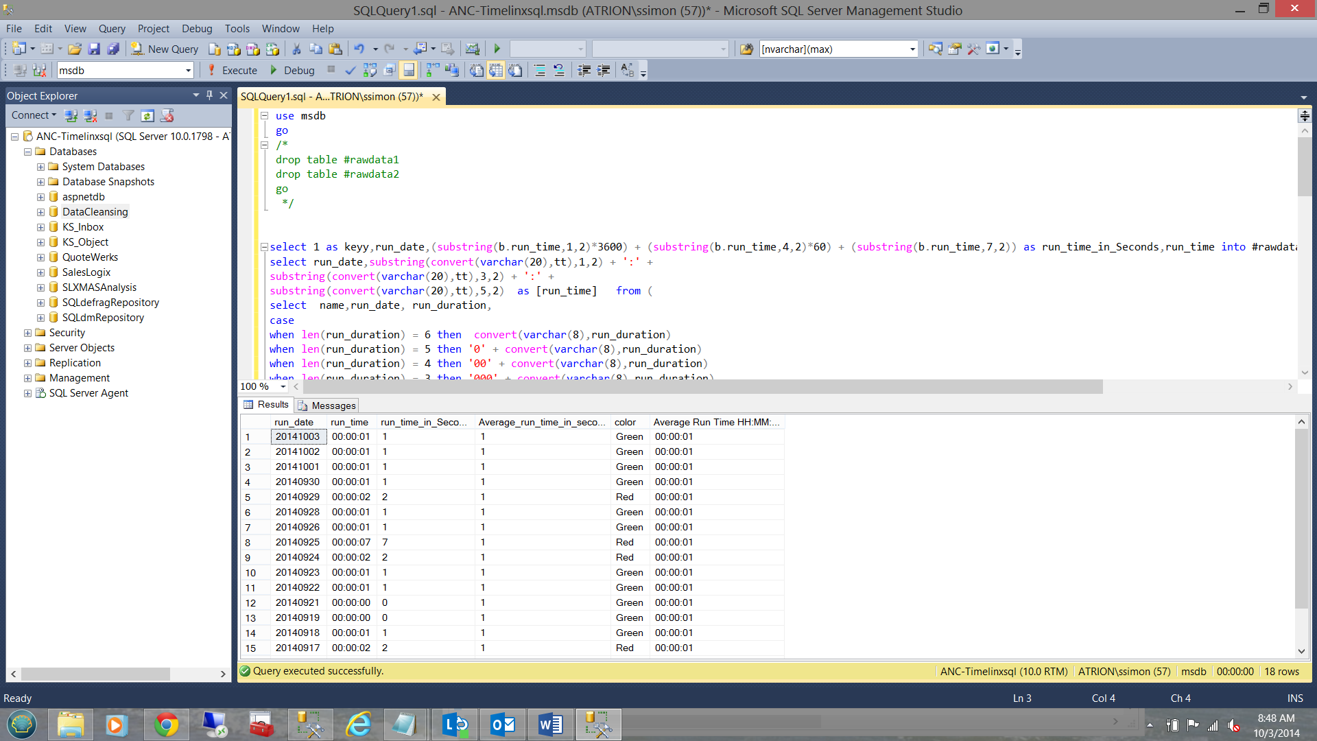
use msdb go /* drop table #rawdata1 drop table #rawdata2 go */ select 1 as keyy,run_date,(substring(b.run_time,1,2)*3600) + (substring(b.run_time,4,2)*60) + (substring(b.run_time,7,2)) as run_time_in_Seconds,run_time into #rawdata1 from ( select run_date,substring(convert(varchar(20),tt),1,2) + ':' + substring(convert(varchar(20),tt),3,2) + ':' + substring(convert(varchar(20),tt),5,2) as [run_time] from ( select name,run_date, run_duration, case when len(run_duration) = 6 then convert(varchar(8),run_duration) when len(run_duration) = 5 then '0' + convert(varchar(8),run_duration) when len(run_duration) = 4 then '00' + convert(varchar(8),run_duration) when len(run_duration) = 3 then '000' + convert(varchar(8),run_duration) when len(run_duration) = 2 then '0000' + convert(varchar(8),run_duration) when len(run_duration) = 1 then '00000' + convert(varchar(8),run_duration) end as tt from dbo.sysjobs sj with (nolock) inner join dbo.sysjobHistory sh with (nolock) on sj.job_id = sh.job_id where name = ‘ANC_DWProjectManagementAvgTimeToStartProject’ and [Message] like '%The job%') a ) b select 1 as Keyy, run_time_in_Seconds into #rawdata2 from #rawdata1 select rd1.run_date, rd1.run_time, rd1.run_time_in_Seconds ,Avg(rd2.run_time_in_Seconds) as Average_run_time_in_seconds, case when Convert(decimal(10,1),rd1.run_time_in_Seconds)/Avg(rd2.run_time_in_Seconds)<= 1.2 then 'Green' when Convert(decimal(10,1),rd1.run_time_in_Seconds)/Avg(rd2.run_time_in_Seconds)< 1.4 then 'Yellow' else 'Red' end as [color], case when len(convert(varchar(2),Avg(rd2.run_time_in_Seconds)/(3600))) = 1 then '0' + convert(varchar(2),Avg(rd2.run_time_in_Seconds)/(3600)) else convert(varchar(2),Avg(rd2.run_time_in_Seconds)/(3600)) end + ':' + case when len(convert(varchar(2),Avg(rd2.run_time_in_Seconds)%(3600)/60)) = 1 then '0' + convert(varchar(2),Avg(rd2.run_time_in_Seconds)%(3600)/60) else convert(varchar(2),Avg(rd2.run_time_in_Seconds)%(3600)/60) end + ':' + case when len(convert(varchar(2),Avg(rd2.run_time_in_Seconds)%60)) = 1 then '0' + convert(varchar(2),Avg(rd2.run_time_in_Seconds)%60) else convert(varchar(2),Avg(rd2.run_time_in_Seconds)%60) end as [Average Run Time HH:MM:SS] from #rawdata2 rd2 inner join #rawdata1 rd1 on rd1.keyy = rd2.keyy group by run_date,rd1.run_time ,rd1.run_time_in_Seconds order by run_date desc |
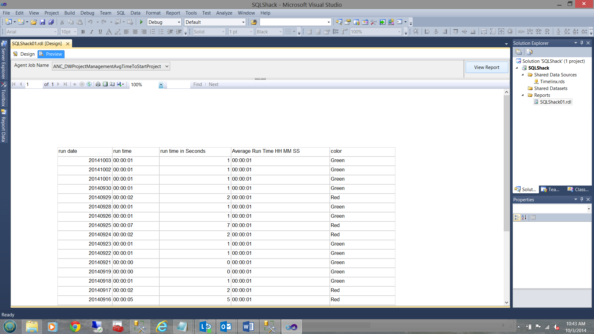
When run, the code generates the following results:
Creating our monitoring project
As a starting point, I create a Reporting Services project within Visual Studio Development tools, with a shared data connection through to our SQL Server.
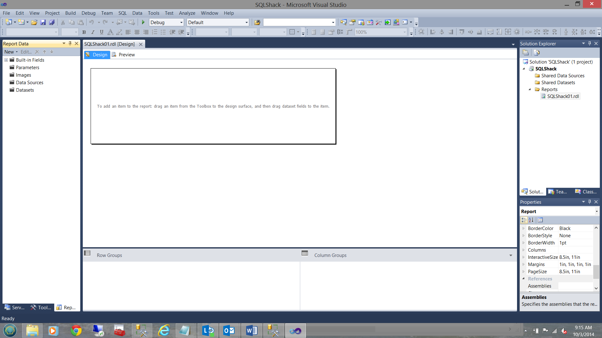
Our database connection looks as follows:
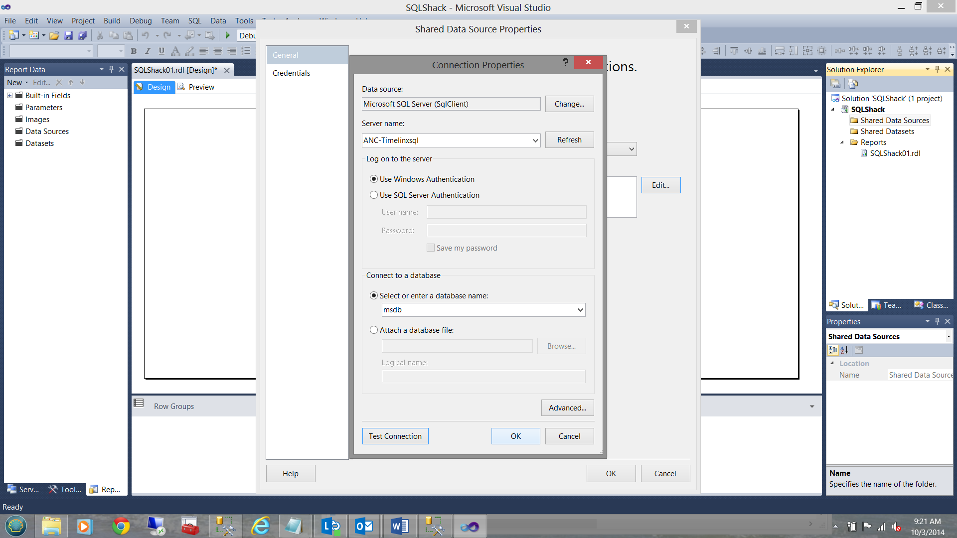
Note that I have selected MSDB as my database, as the DMVs reside within this database.
As I want my dashboard to be as flexible as possible, I want the user to have the freedom to select the job of his or her choice.
This said, what I need is a list of relevant agent jobs on my server.
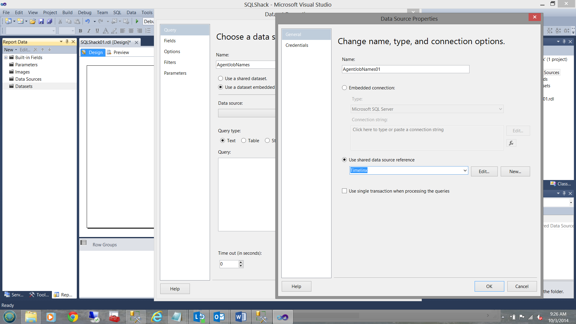
To create this list I now create a dataset to ‘store’ these job names. I create a ‘local’ data source from the shared data source ‘Timelinx’(created in a previous step). This data will be accessed via a report parameter (discussed below):
The code to populate this list is fairly straight forward and may be seen below:
|
1 2 3 4 5 6 |
select systemjobs.name as 'Agent Job Name' from msdb.dbo.sysjobs systemjobs left join master.sys.syslogins systemlogin on systemjobs.owner_sid = systemlogin.sid |
My ‘create a data set’ screen is shown below:
My completed dataset now appears under the Dataset tab on the left (as seen below):
This said and done, I now need to define a parameter to permit the user to select which job he or she wishes to view.
Creating our job parameter
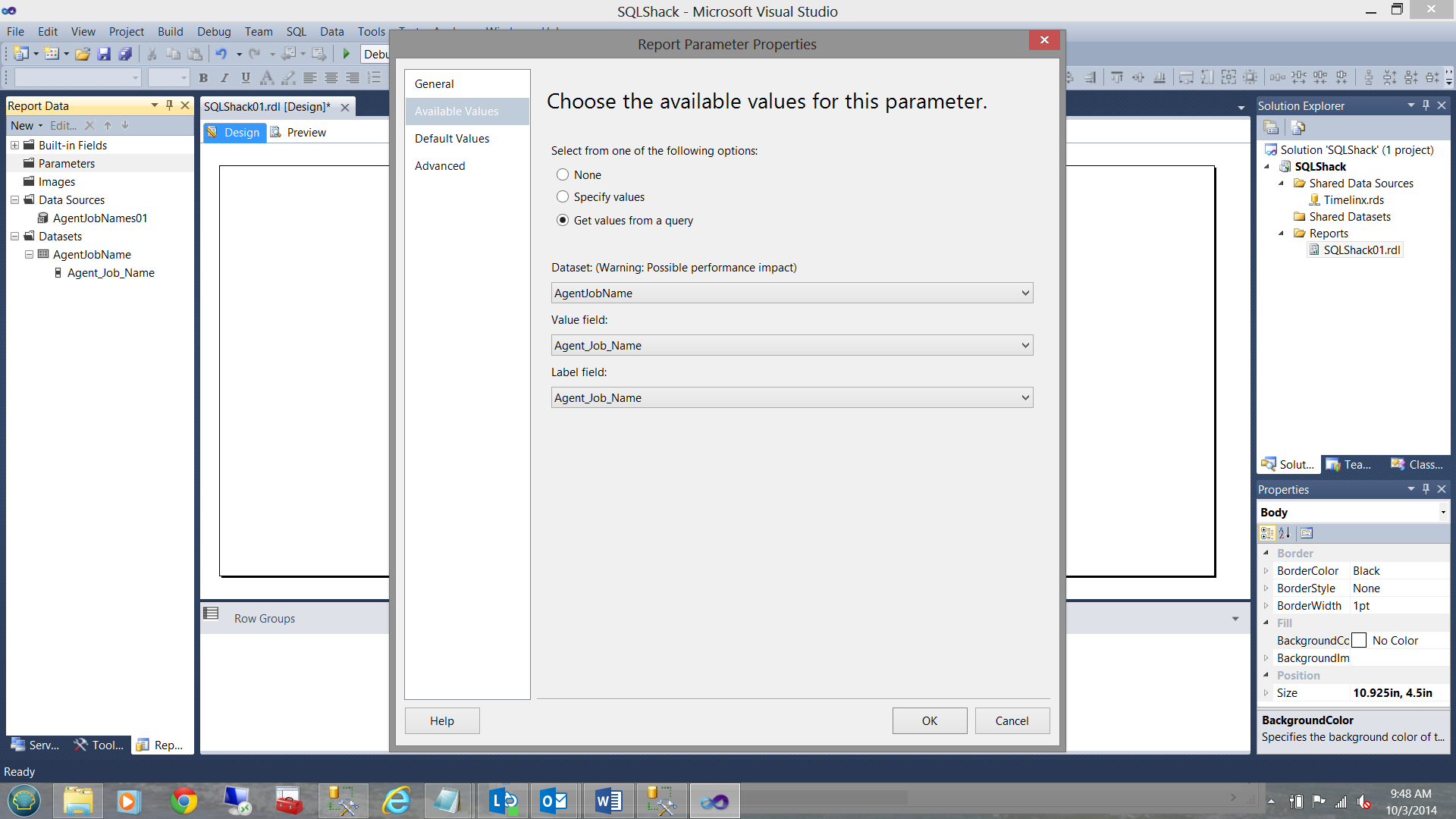
Declaring a parameter is quick and fairly simple. The data for the parameter will be obtained from the dataset that we just created. The completed parameter definition is shown below:
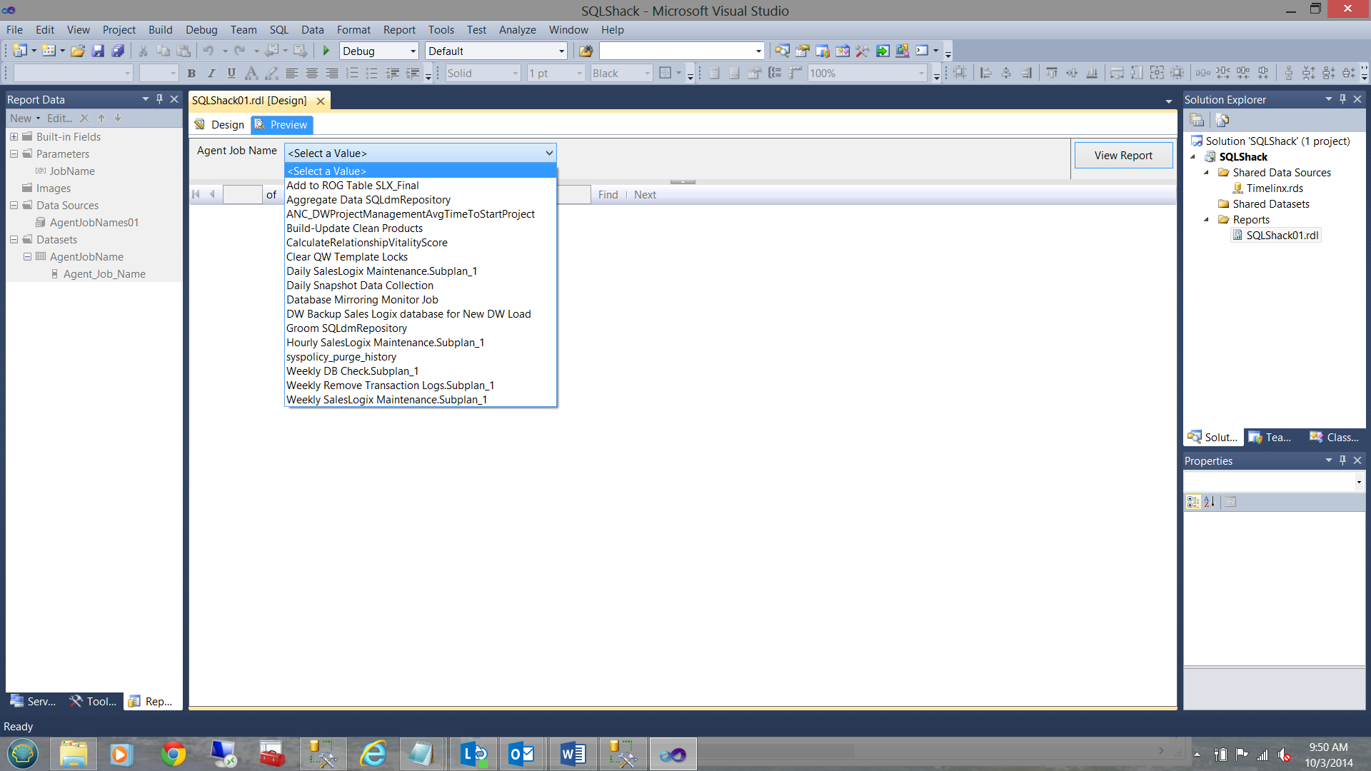
I can now preview the contents of my ‘Jobs’ dataset, to select the name of the job that I am interested in examining:
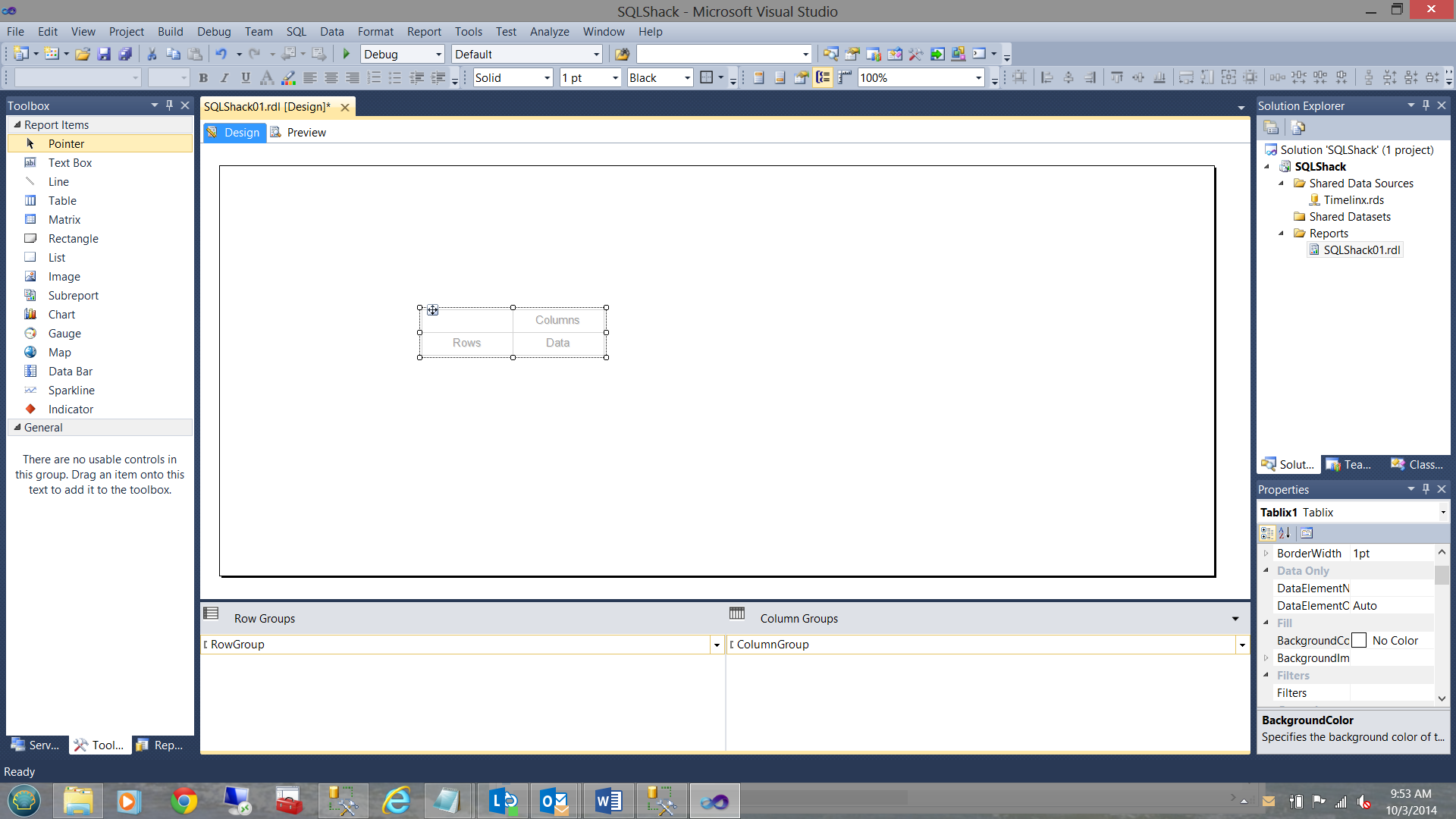
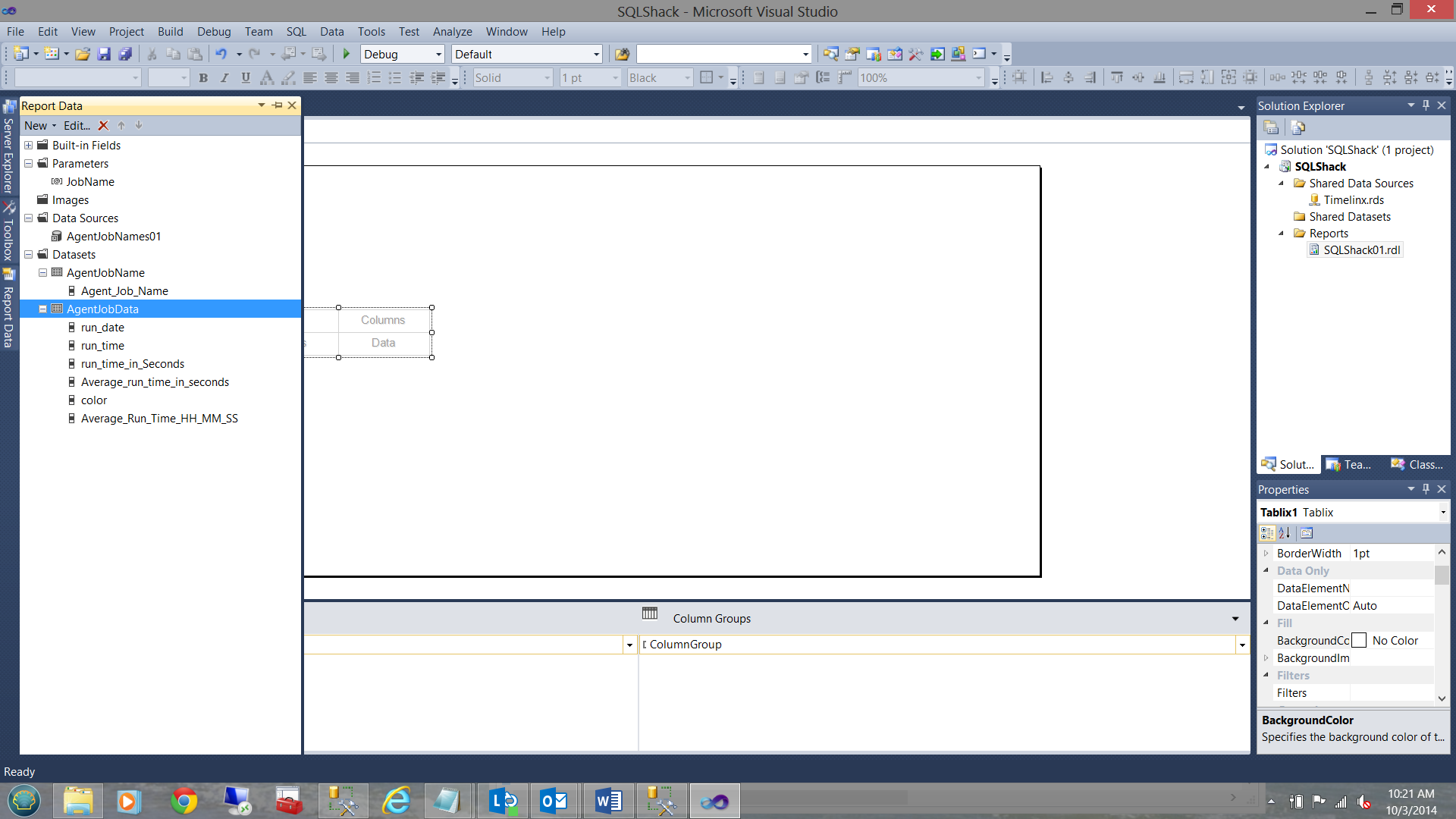
Now this is ‘fine and dandy’ however in order to actually view the data (relevant to the actual job), we must incorporate a matrix onto our drawing surface:
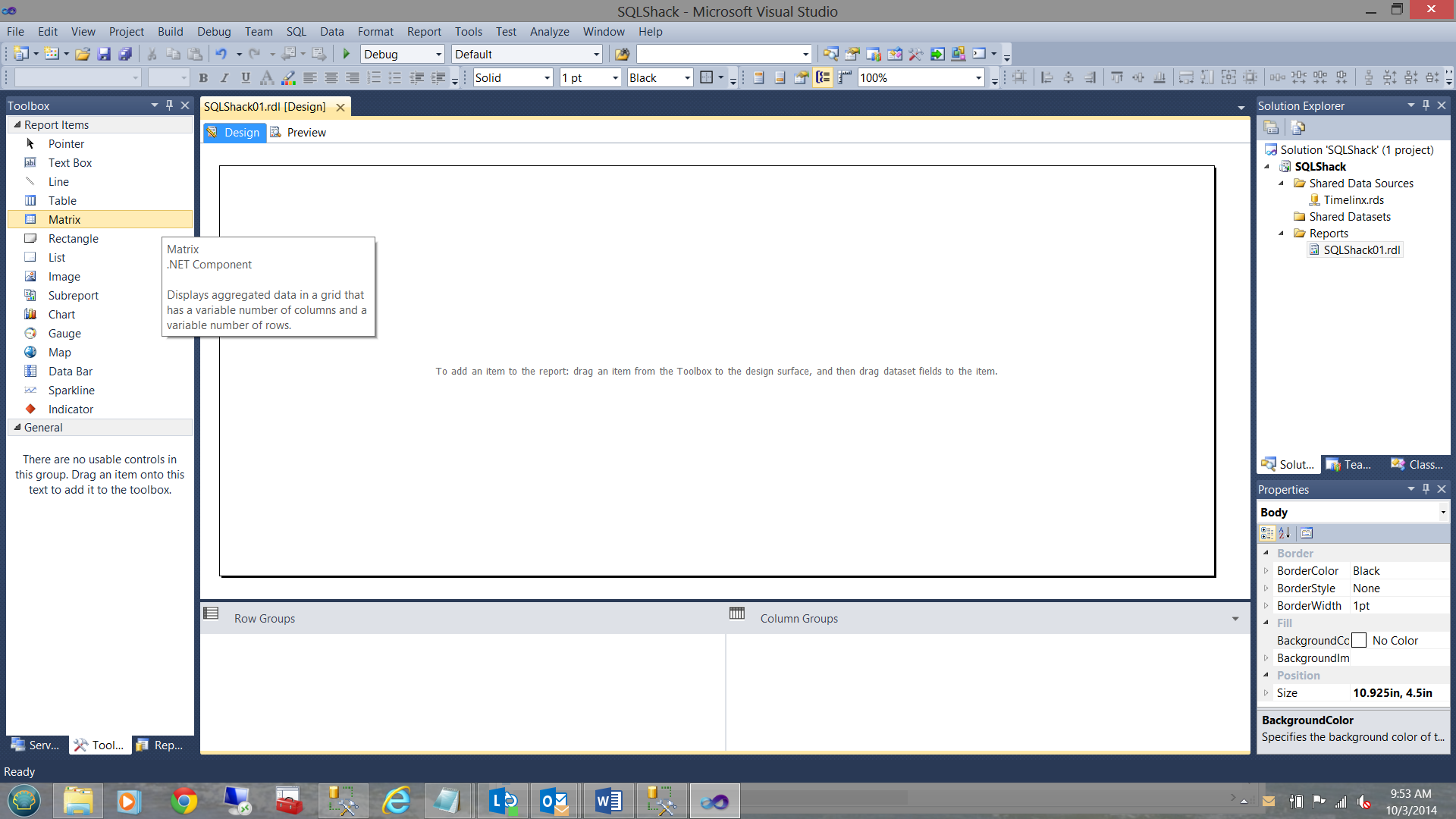
Our matrix appears as follows:
Our next task is to define the dataset that will contain the results for our matrix. There are numerous ways of obtaining the necessary data including the creation of a stored procedure and using native T-SQL code.
While I normally use a stored procedure (which is more efficient), in this case most of the results are coming from MSDB and I am averse to creating a stored procedure within that system database.
Now, there are workarounds that one can do to ‘compile’ the stored procedure from another database and yet trick it into thinking that it is in fact being created from within the proper MSDB region.
However this is not for the scope of this article.
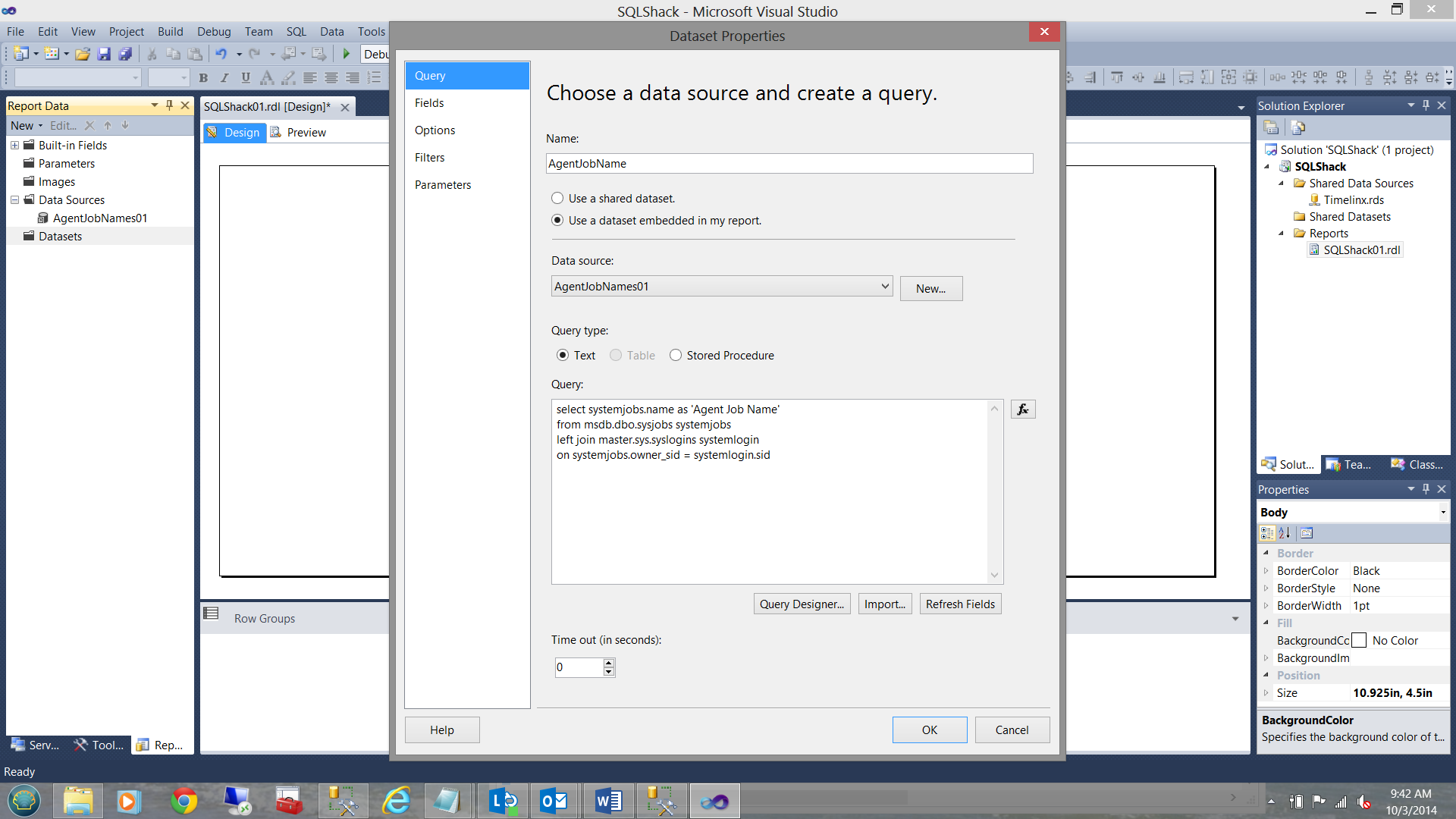
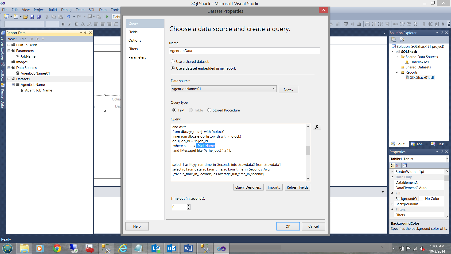
This said, I enclose the code within the ‘Query Text Box’.
Further, note the parameter(@JobName) inserted for the job name (see below):
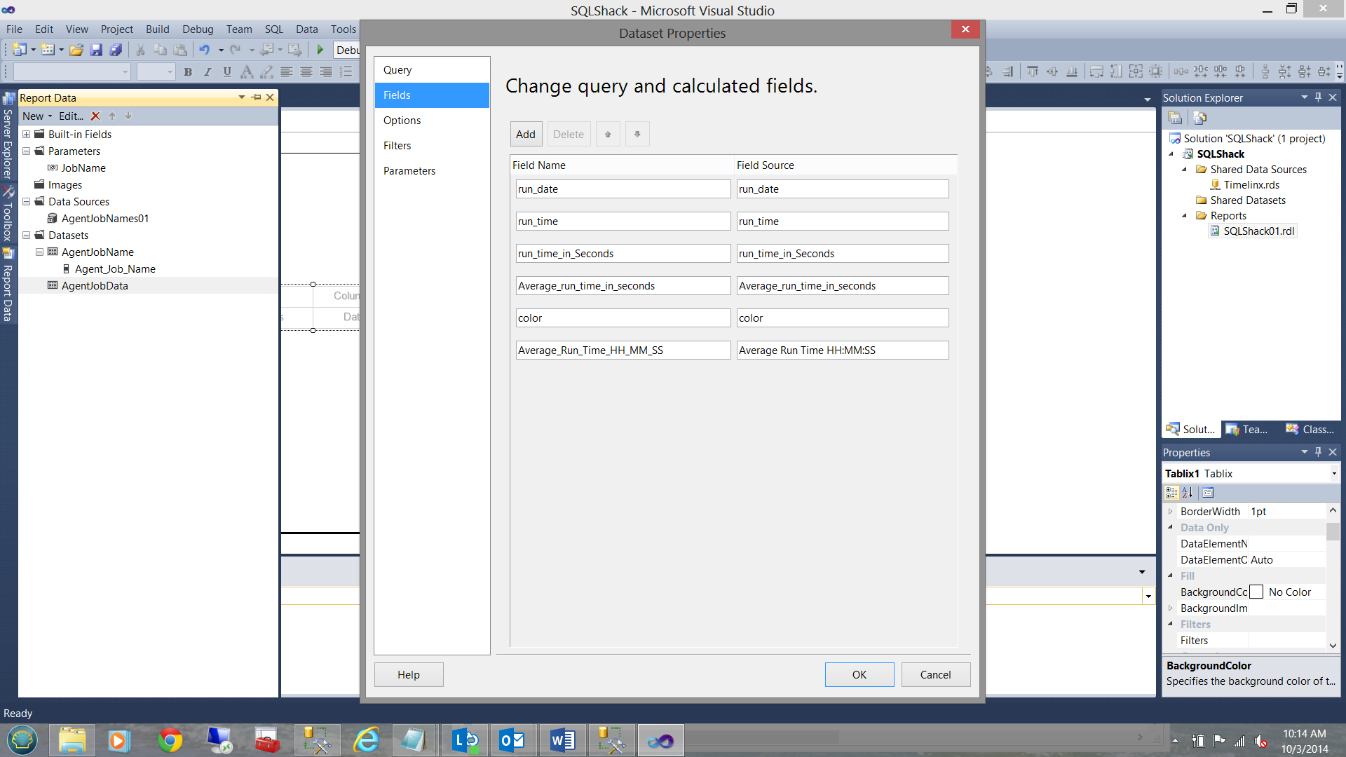
I now click the ‘Refresh Fields’ button on the screen above to ensure that all my fields will be extracted. Going to the ‘Fields’ tab on the left hand side of my dataset screen, I click the ‘Fields’ button and note the fields that will be extracted:
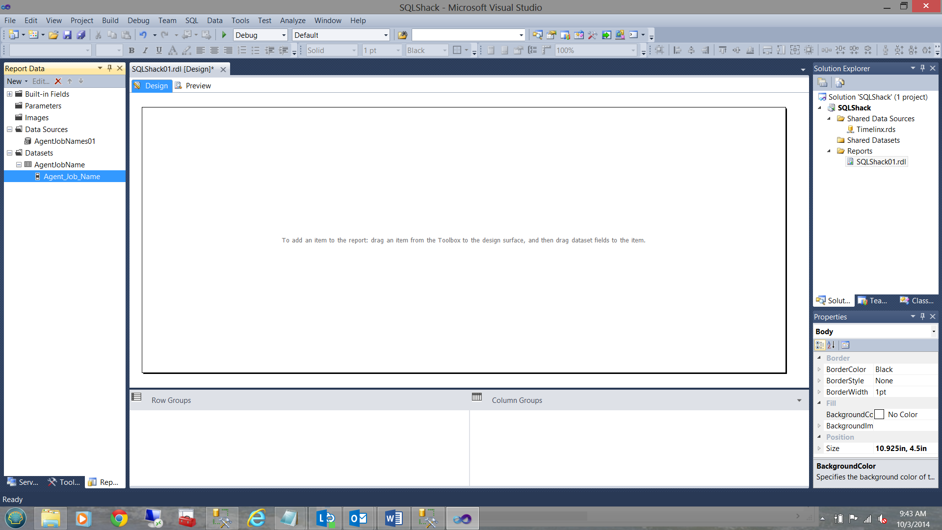
Once I click ‘OK’ to complete, my work surface should show our newly created dataset as follows:
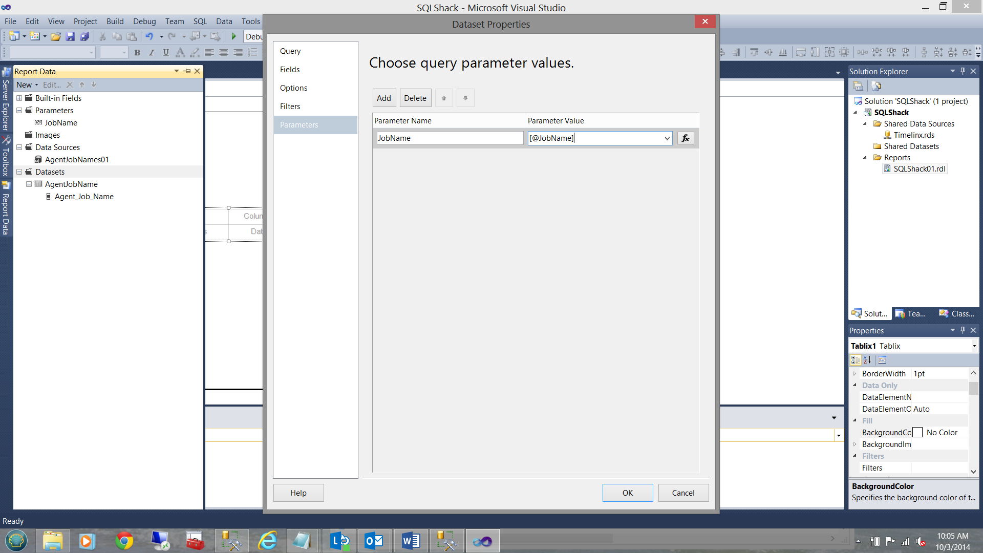
Connecting the parameter value to the dataset query
This done, I click on the parameter tab to complete the process, by letting the dataset know that a parameter is necessary to complete my query AND that that parameter will be selected by the end user:
Upon completion of this step, we shall note that we now have two datasets. One contains a list of the ‘Agent Jobs’ and the other will eventually contain data relevant to the selected job.

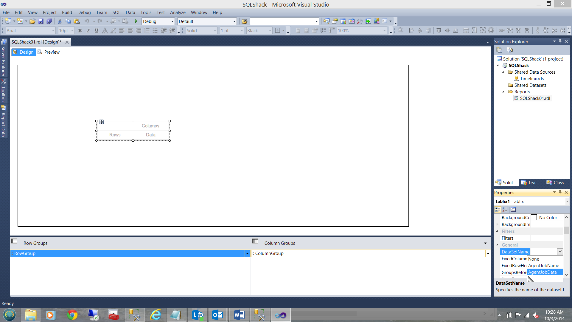
Setting the ‘datasetname’ for the matrix
Let us now set up the matrix by connecting the Matrix’s ‘Data Set Name’ Property to the dataset that we just created. This may be seen in the following screen dump:
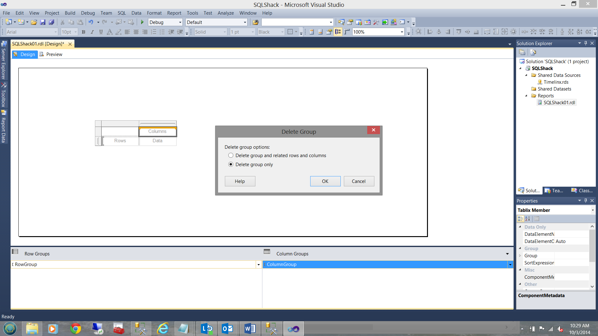
Our last chore is to remove the column grouping from the matrix (as it is not required for our example). Merely right click on the ‘ColumnGroup’ tab and select ‘Delete group only’:
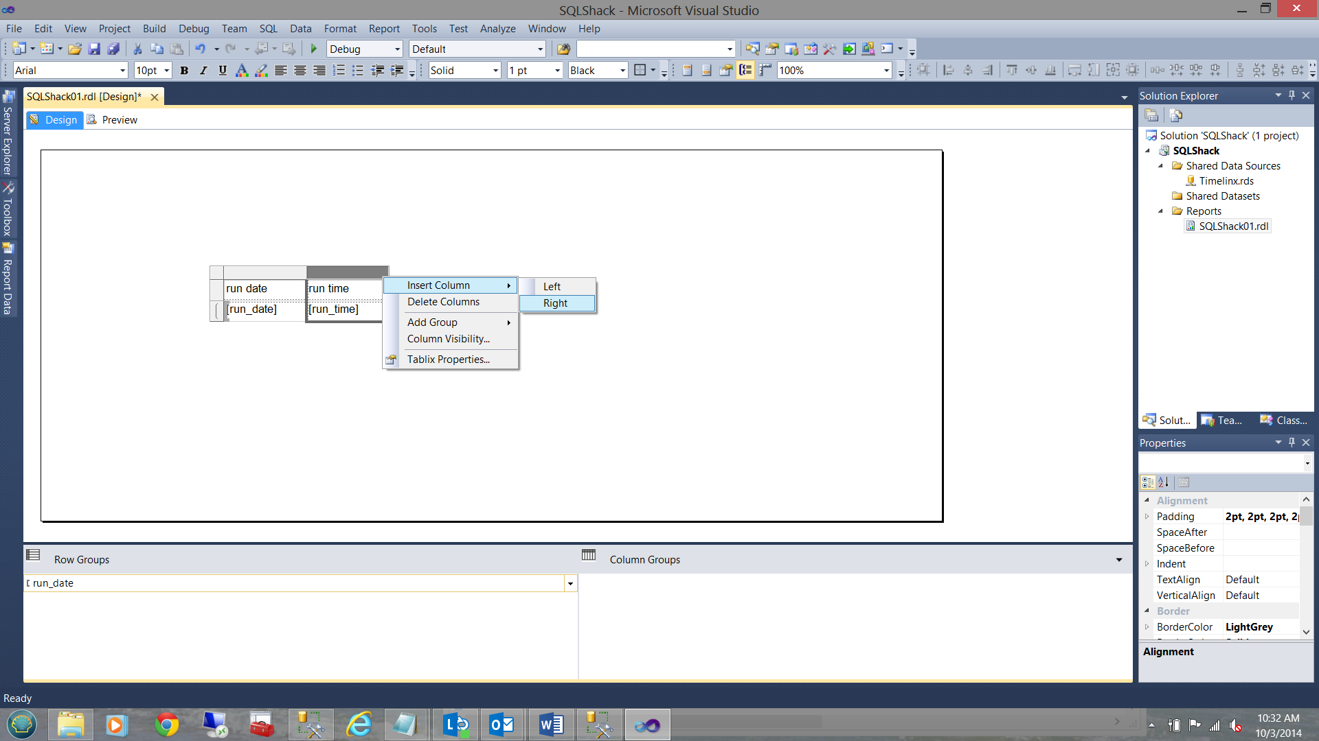
Further I add a few more columns to the matrix through the use of the context menu (right click):
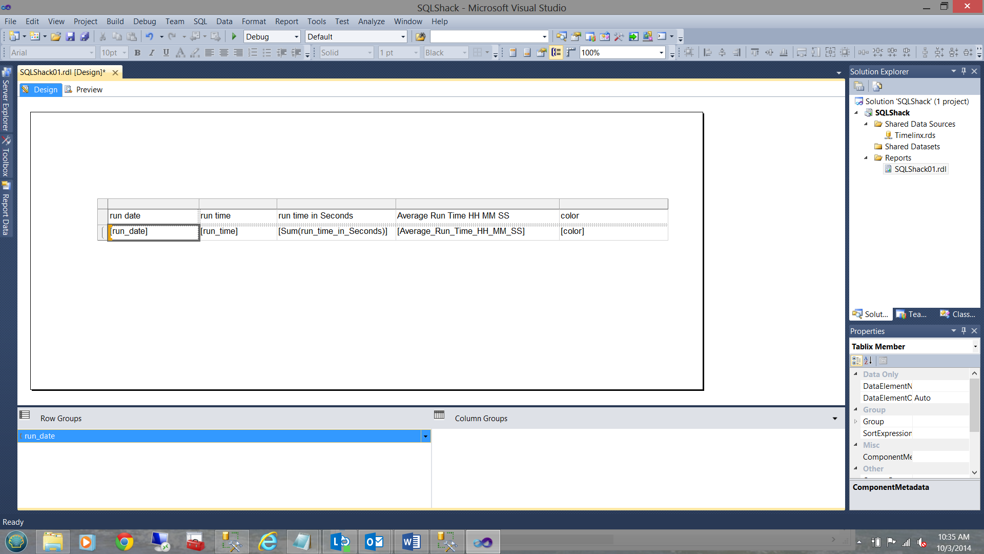
Our completed matrix looks as follows, once fully populated. Note that the grouping is by date:
Sorting our data
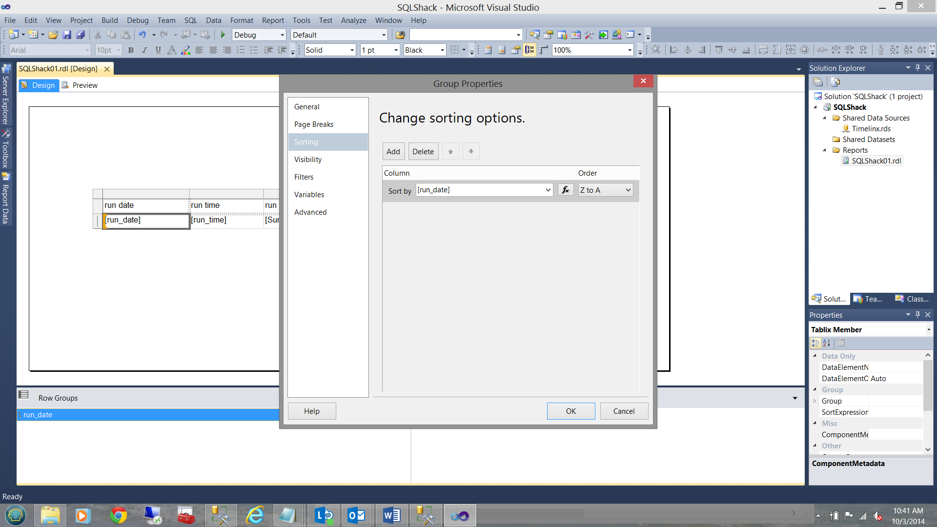
As I wish to have run dates in descending order, i.e. my most recent run at the top of the list, I right click on the ‘run_date’ grouping (highlighted above) and select the sorting option and order it from ‘Z-A’ as shown below:
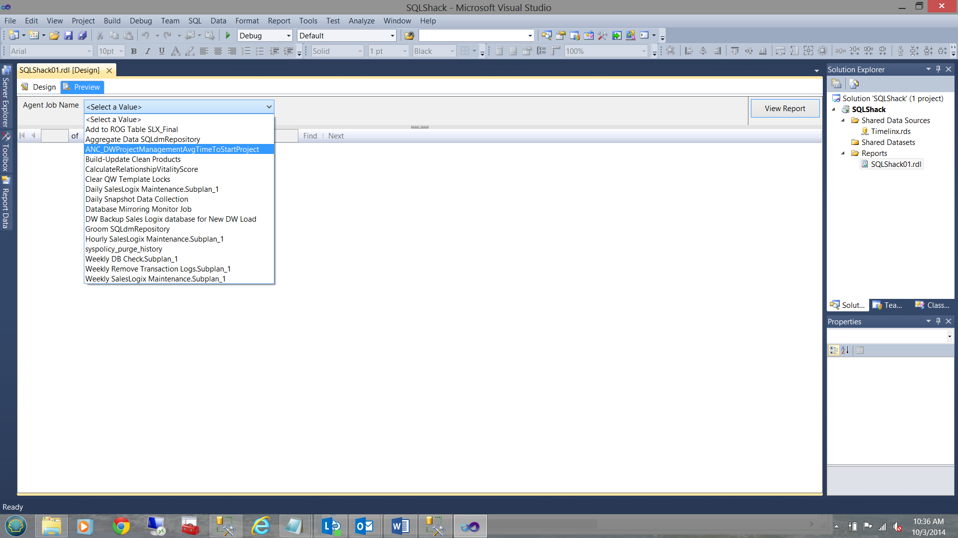
Now running the query, I obtain the following results. First my selection screen:
The screen dump below shows the returned dataset:
Adding the eye candy
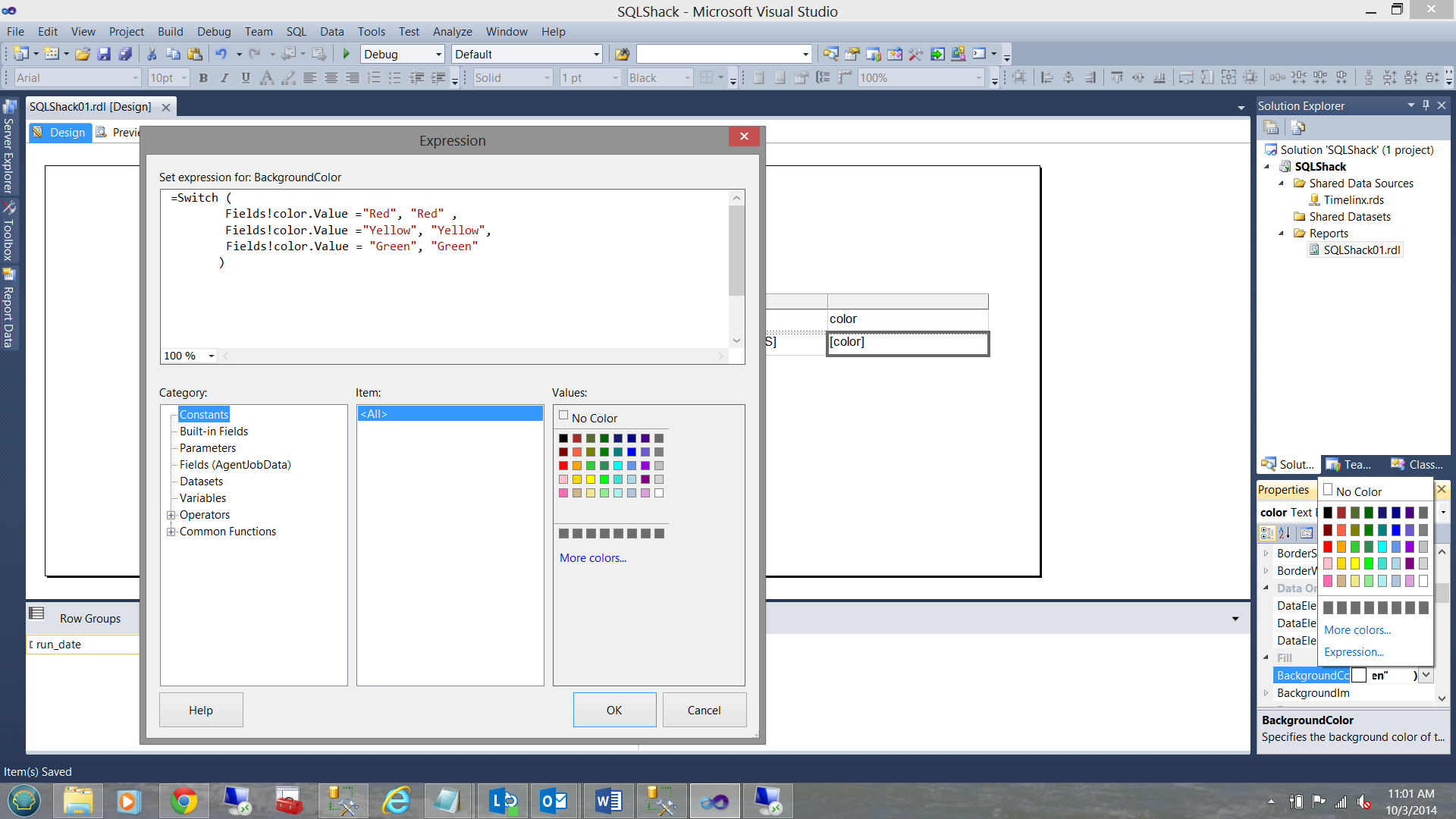
With the skeleton of our report now complete, we need to add a bit of ‘oomph’ to report, highlighting anomalies. The solution that I utilized for this example was to use the appropriate fill for the ‘color’ field. I use a switch constraint to achieve this goal:
|
1 2 3 4 5 6 7 |
=Switch ( Fields!color.Value ="Red", "Red" , Fields!color.Value ="Yellow", "Yellow", Fields!color.Value = "Green", "Green" ) |
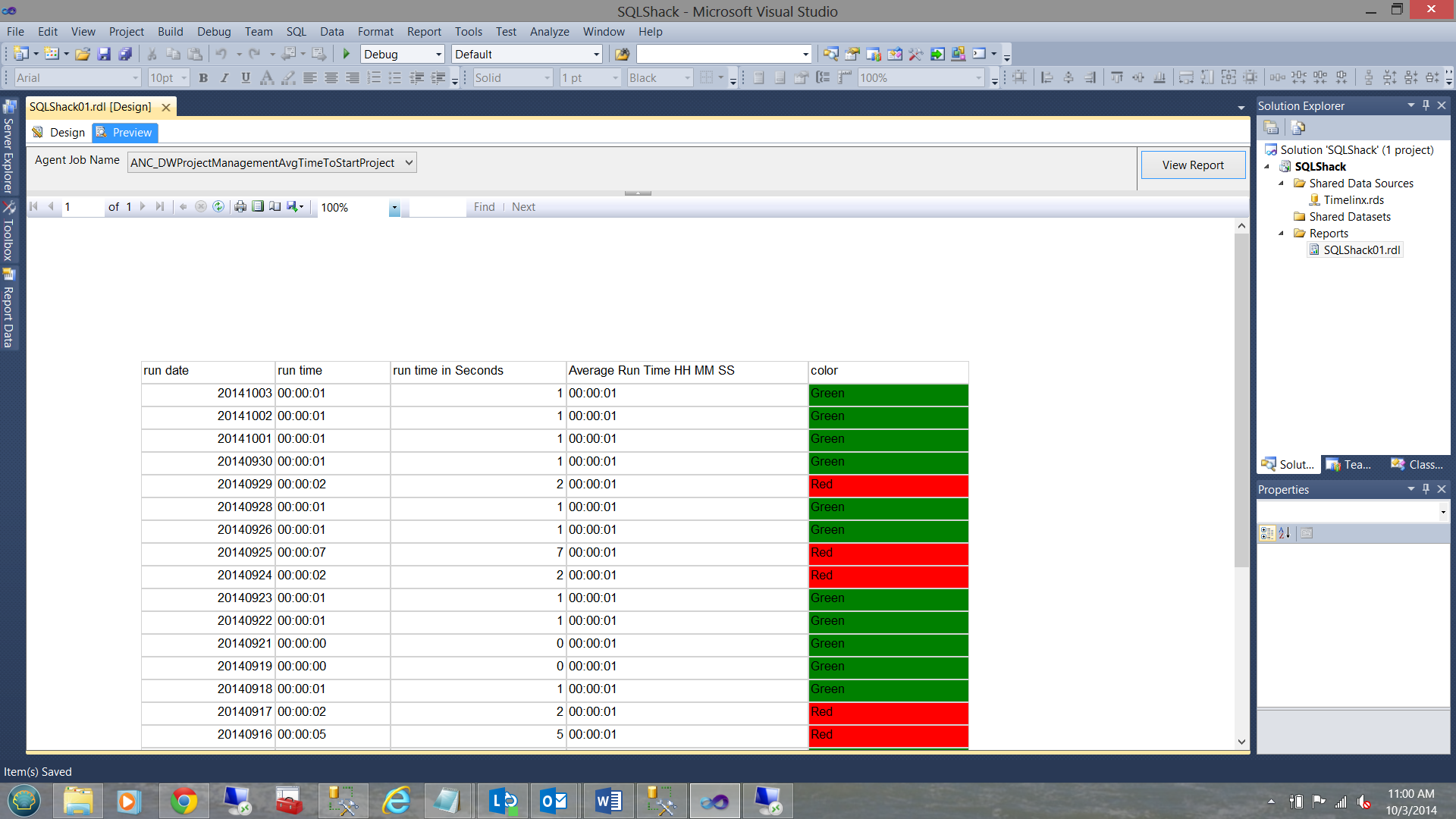
When run, the results become immediately apparent, as shown below:
It should be noted that there are certainly other ways of achieving the same results. Examples are through calculations made at run time and it is left up to the reader to try for themselves.
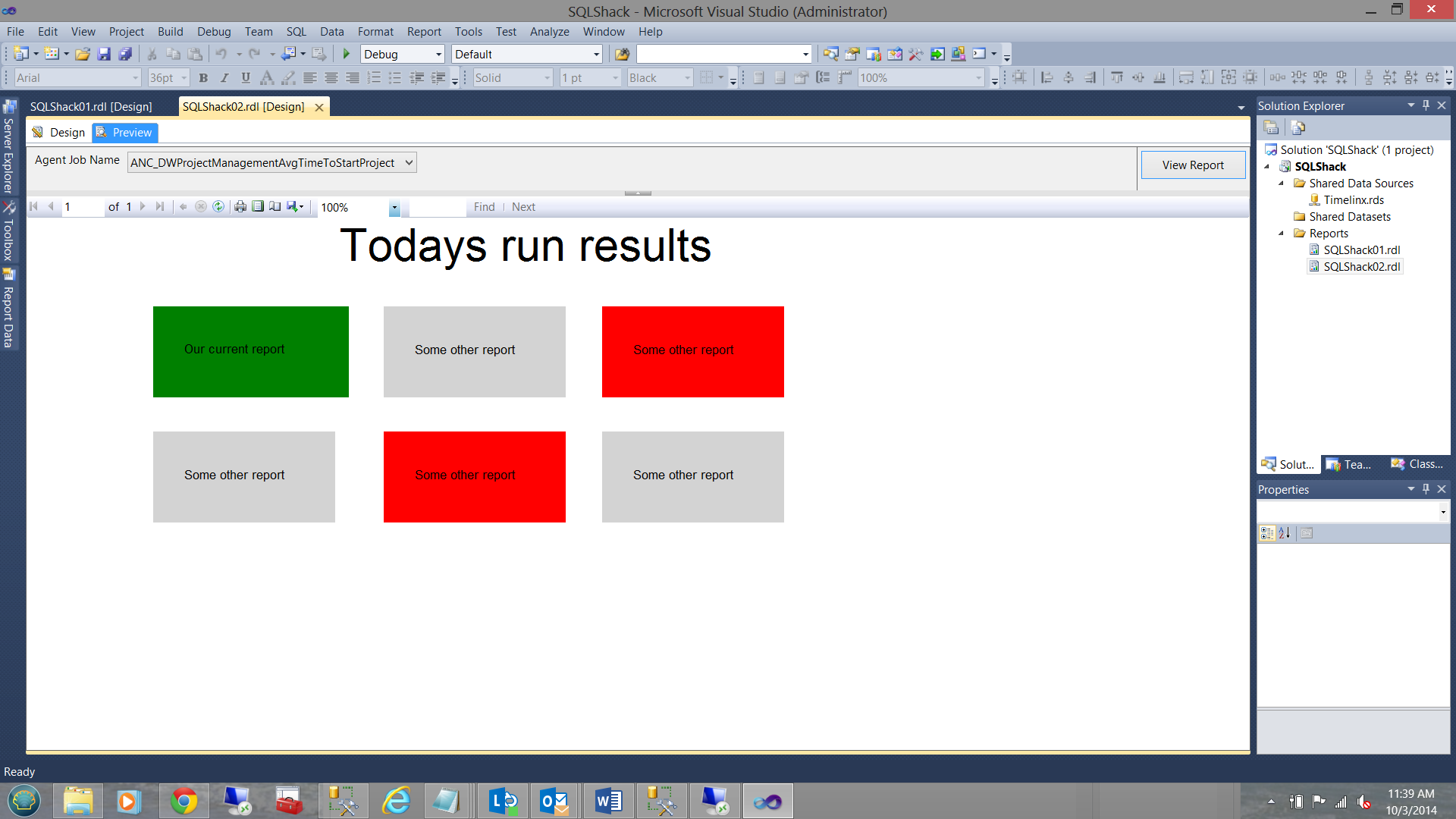
A final touch would be to show only the results for the latest run. In reality this would be done as a part of a series of report ‘blocks’ and is shown fully completed in the following screen dumps.
Creating a full monitoring dashboard based upon what we have just developed
For our last example I created a report with a series of six rectangles. Five of these are purly for visual effect. The upper left rectangle has had its ‘Fill’ property altered as follows:
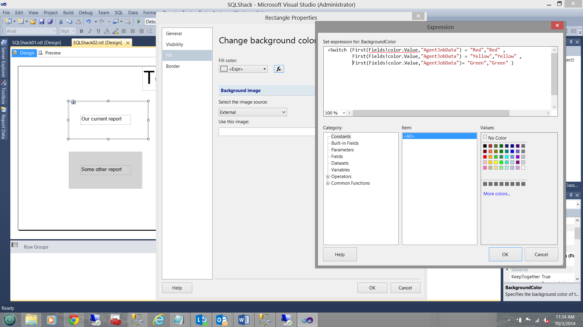
Thus when the report is run, the following is achieved. Note that the latest run today was clear (green). If there had been issues the color would have changed to red.
Conclusion
Having a dashboard similar to the dashboard shown above provides the DBA and developer alike with a quick reaction information system to monitor the server and jobs BEFORE small issues become major fires.
Steve has presented papers at 8 PASS Summits and one at PASS Europe 2009 and 2010. He has recently presented a Master Data Services presentation at the PASS Amsterdam Rally.
Steve has presented 5 papers at the Information Builders' Summits. He is a PASS regional mentor.
View all posts by Steve Simon
- Reporting in SQL Server – Using calculated Expressions within reports - December 19, 2016
- How to use Expressions within SQL Server Reporting Services to create efficient reports - December 9, 2016
- How to use SQL Server Data Quality Services to ensure the correct aggregation of data - November 9, 2016