In an earlier “get together”, we had a quick look at the DAX language and how to construct useful queries. In today’s conversation we shall be concentrating on utilizing the knowledge that we obtained from the earlier article and seeing how these queries may be utilized for “multiple value” query selection criteria (against a tabular database).
Enough said, let us get started!

Getting started

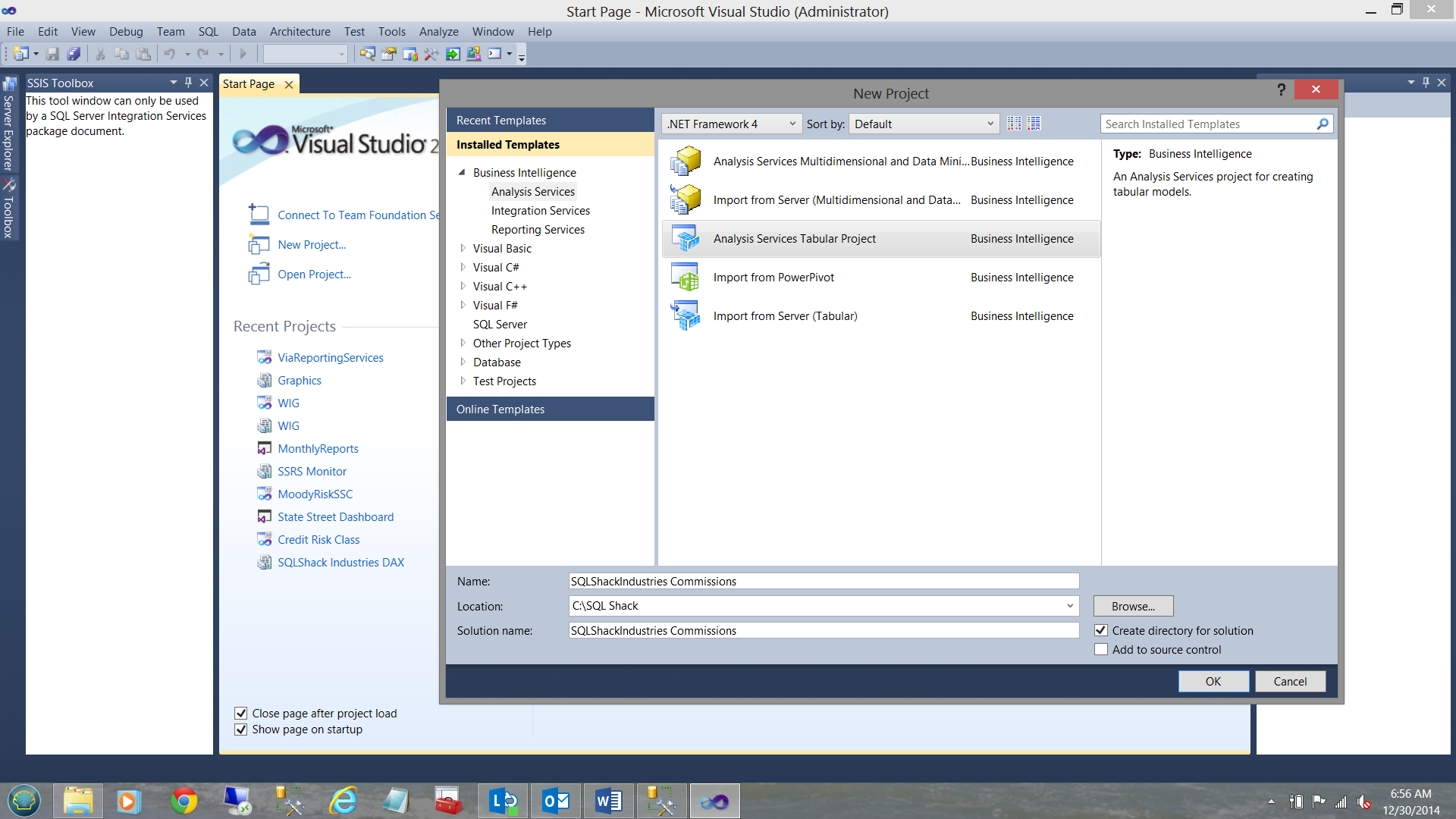
It is said that “Every journey begins with a first step”. We begin by creating a new “Analysis Services Tabular Project” as may be seen below:

Upon clicking “OK” We are asked for the name of the “Workspace server” where our Analysis Services database will be placed (see below).

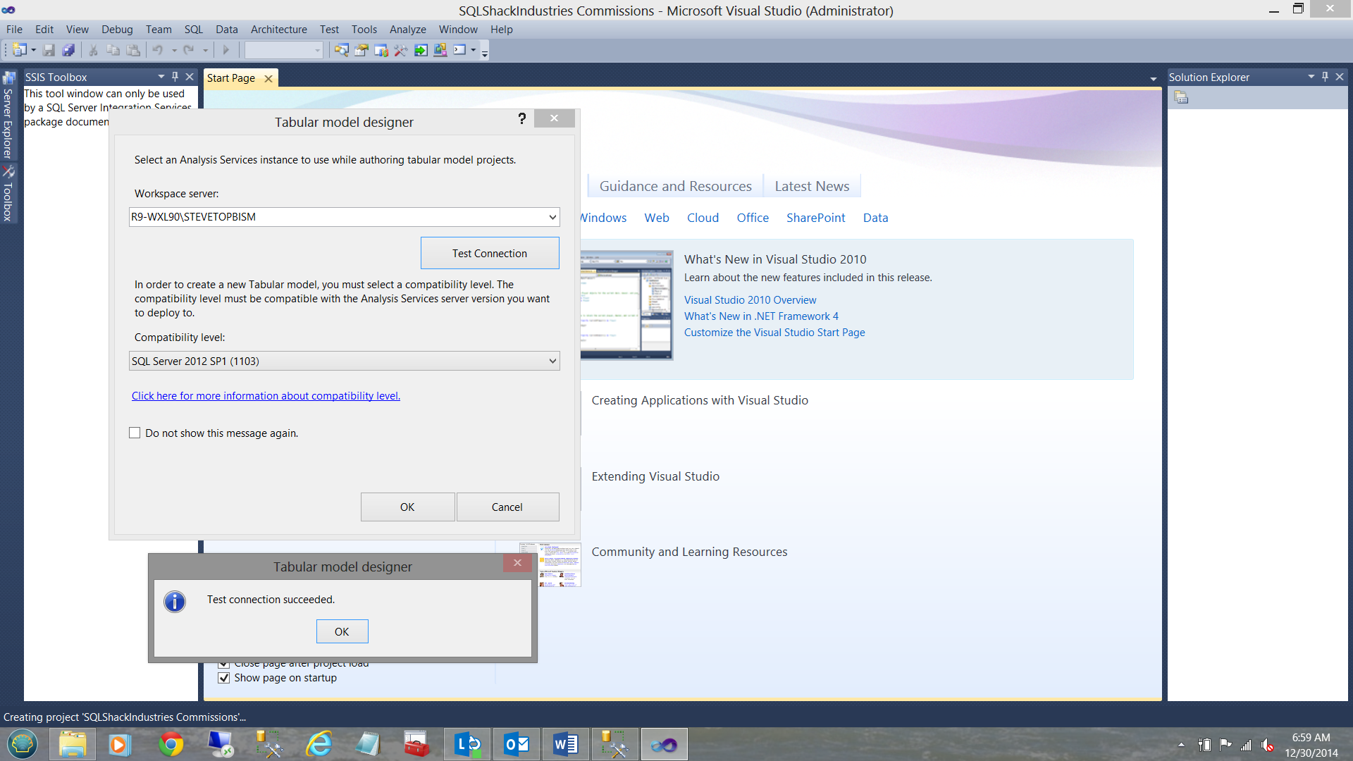
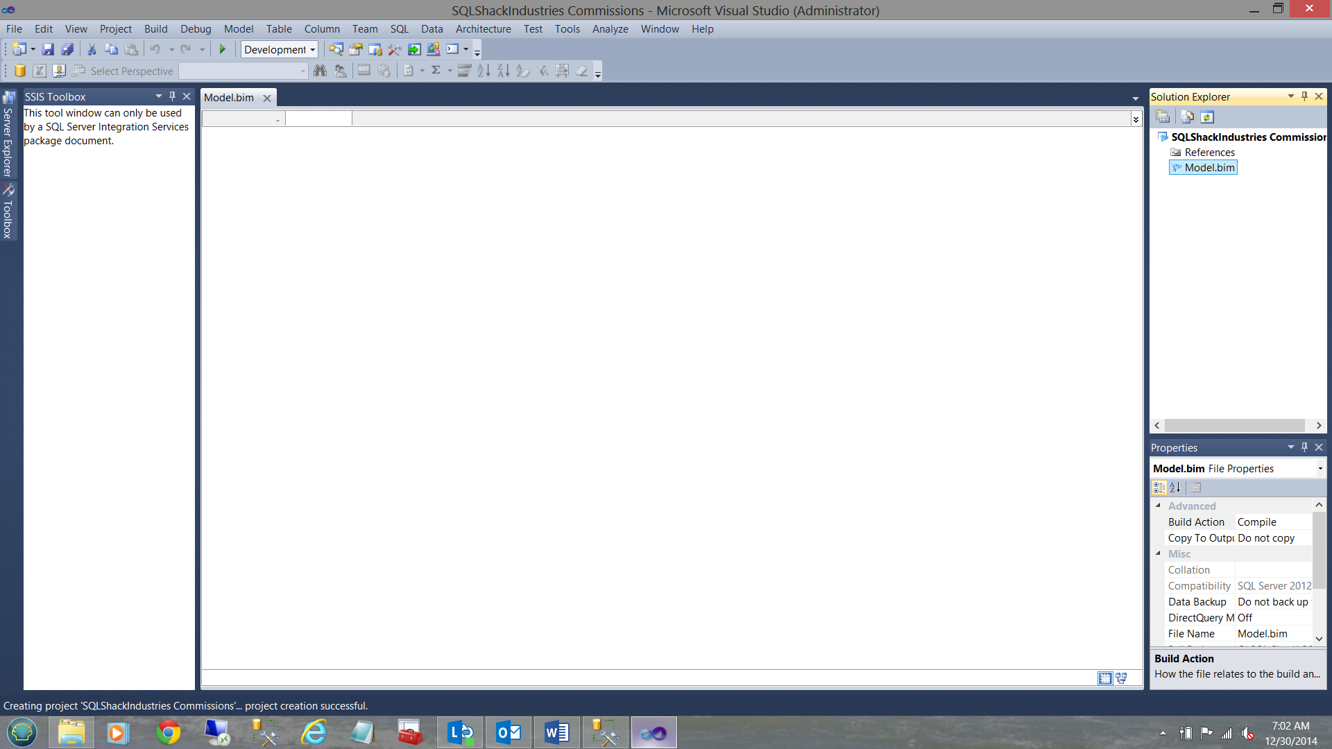
We click OK to close the “Test connection succeeded” box and OK to create the connection. We then find ourselves back on our work surface(see below).

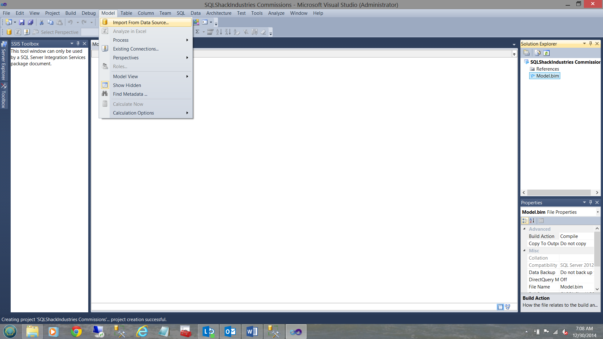
This achieved, we must now configure our Model (BIM = Business Intelligence Model). We now select the Model tab from the ribbon area and “Import from Data Source” (see below).

The “Table Import Wizard” is then brought up (see below).

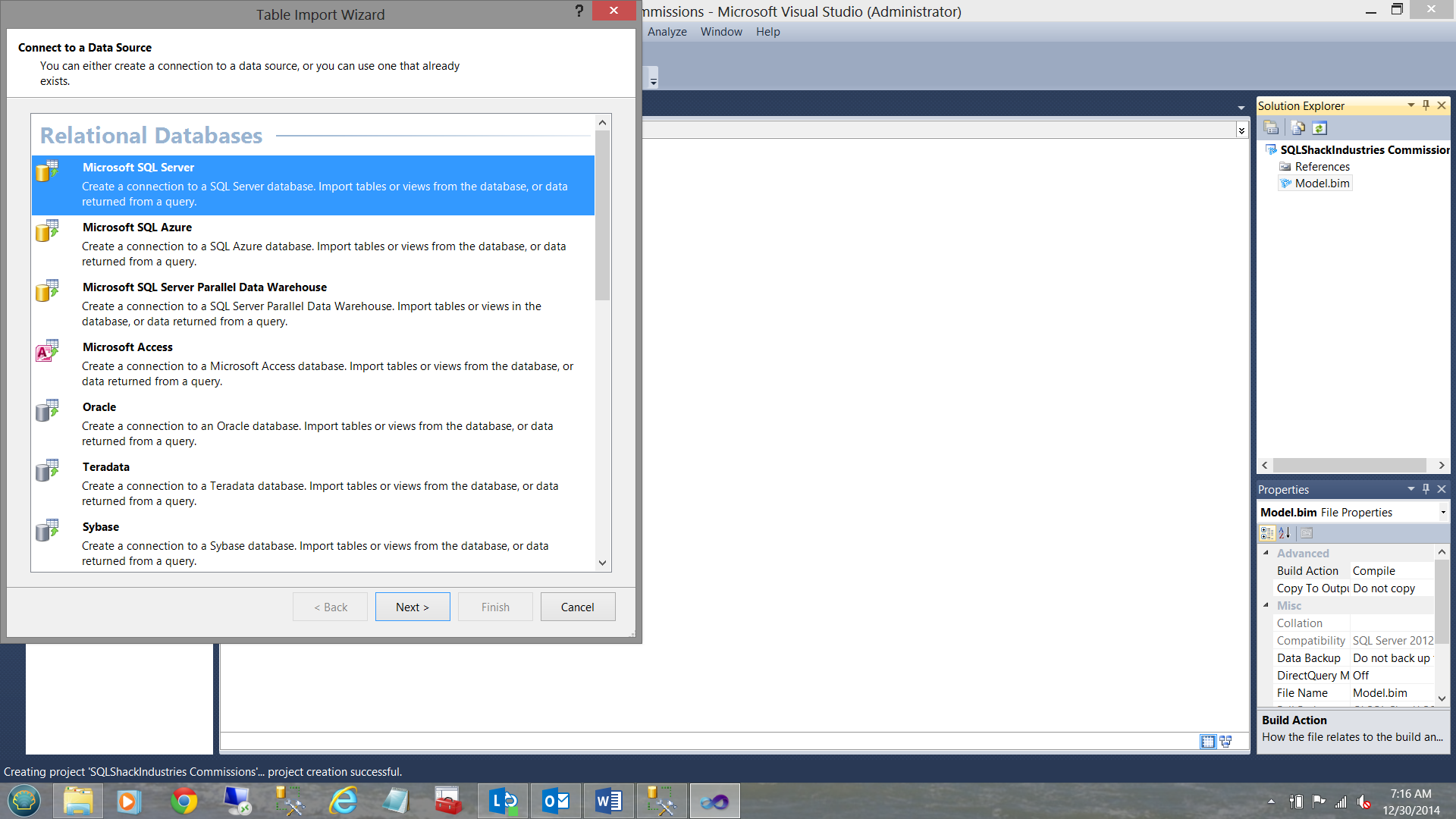
We select “Microsoft SQL Server” from the menu (see above). We click “Next”.

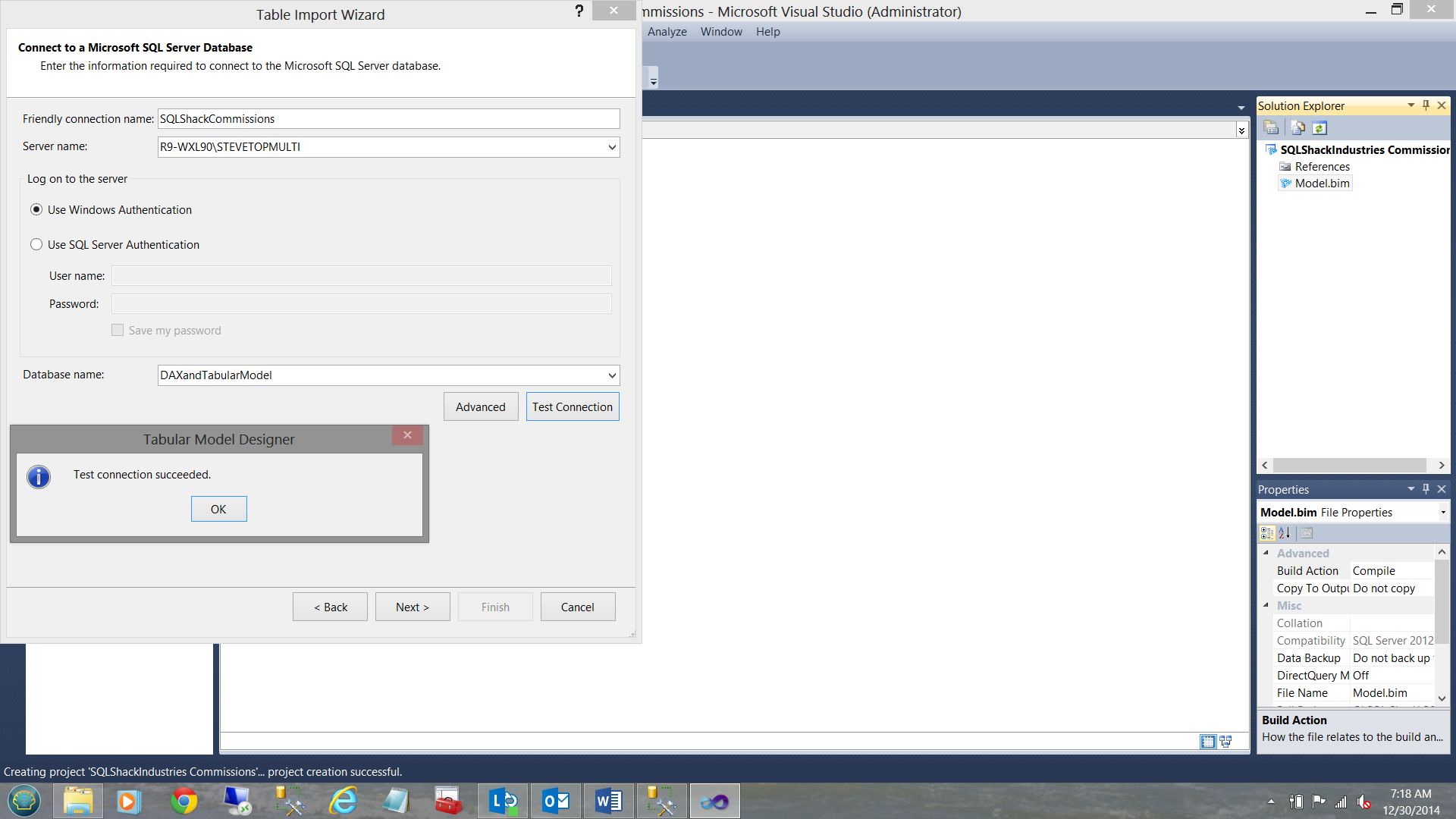
We give our connection a “Friendly connection name” and tell SQL Server Data Tools our source data server name. We test our connection to verify that all is in order (see above). We click “Next”.

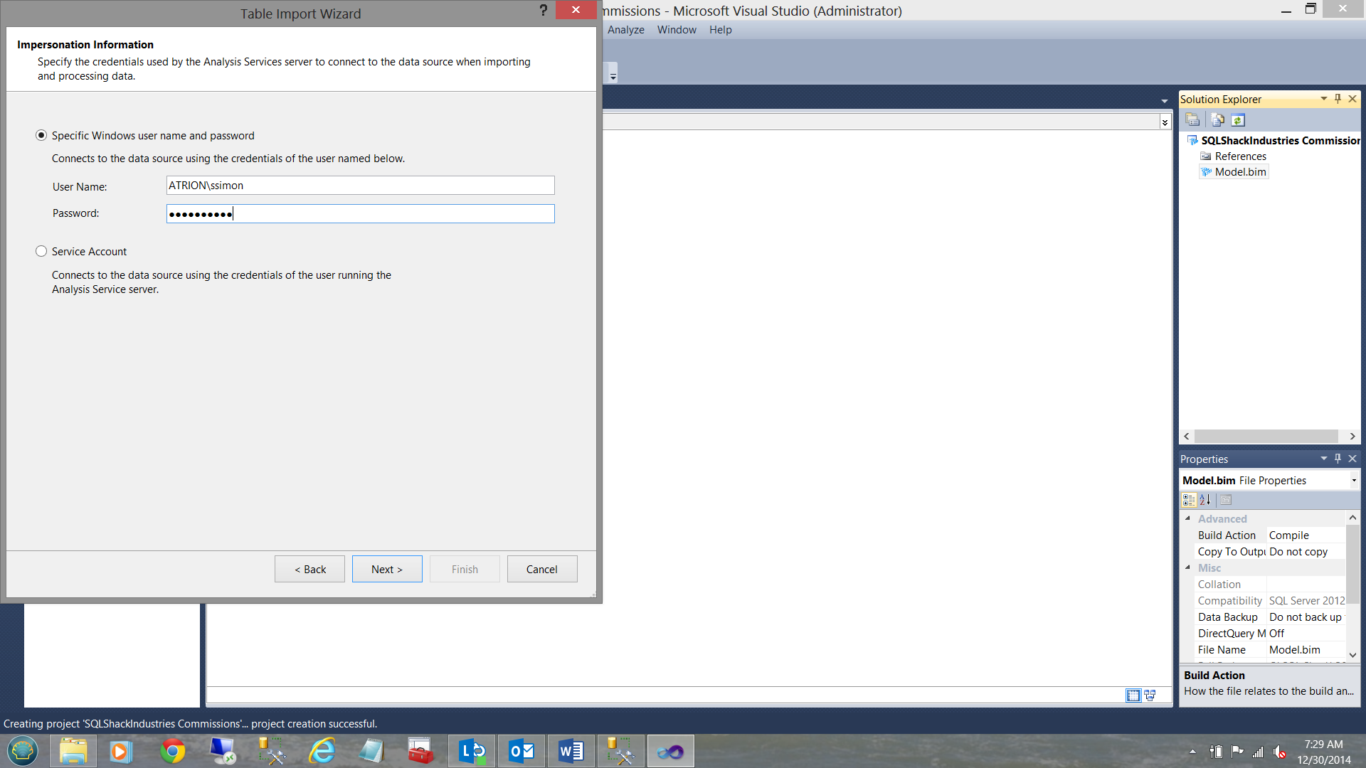
Our credentials are now required (see above). We click “Next”.

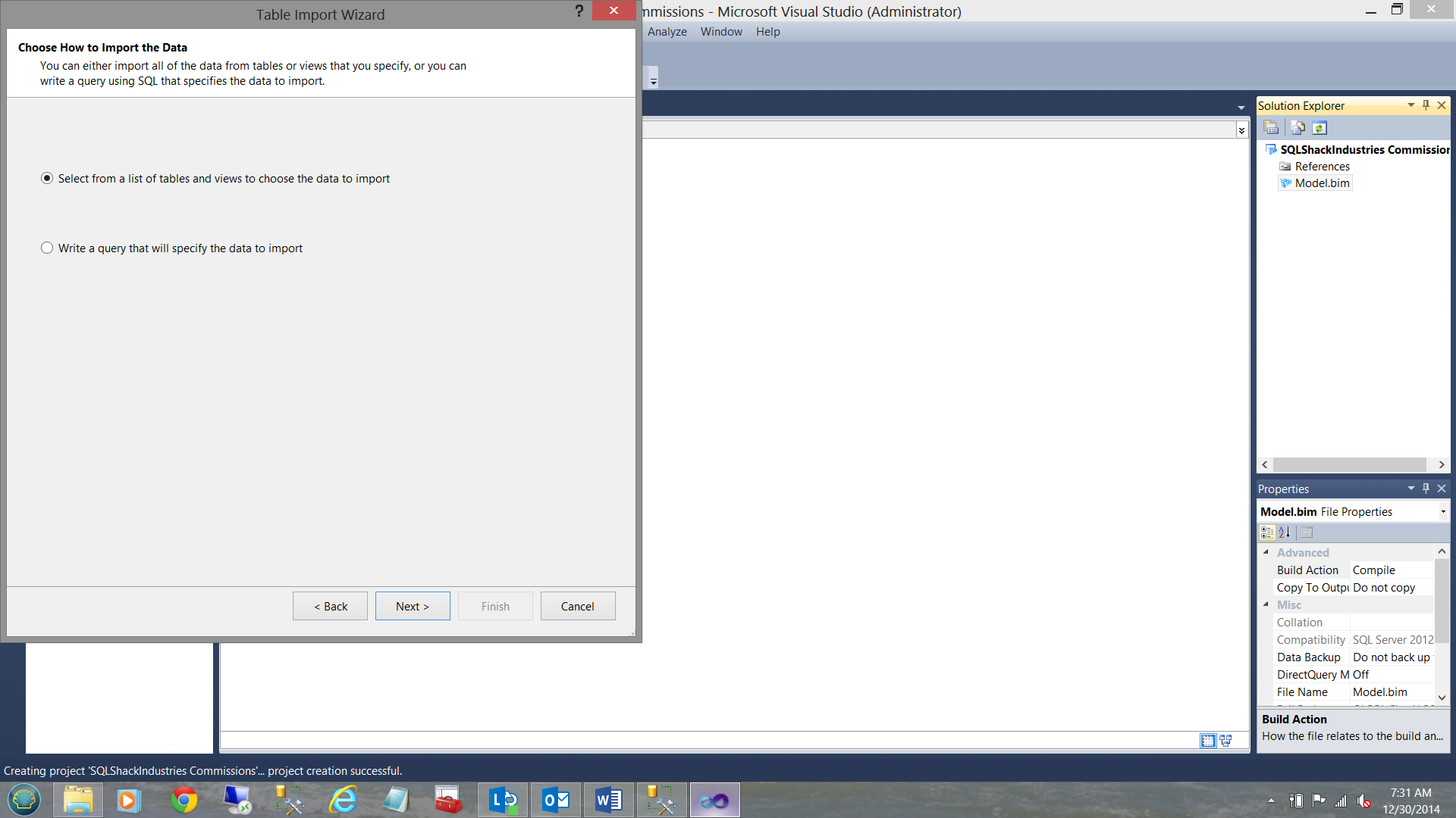
With our credentials in order, we are asked to “Select from a list of tables and views” that will be imported into our data model (see above). Click “Next”.

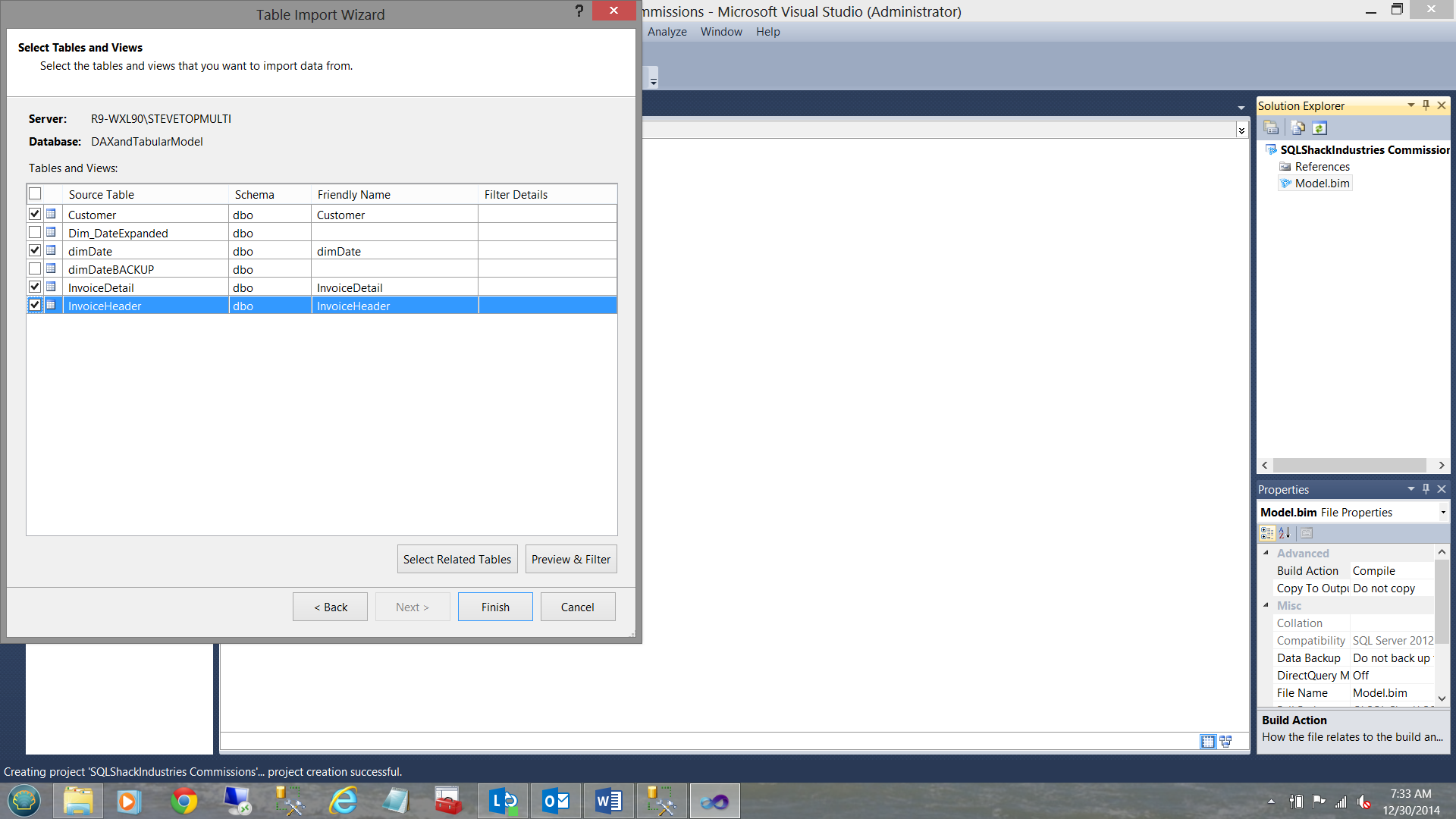
We really only want the Customer, date dimension table (dimDate), the invoice header and invoice detail tables imported (see above). We now click “Finish”.

The loading of the data from the relational tables begins (see above).

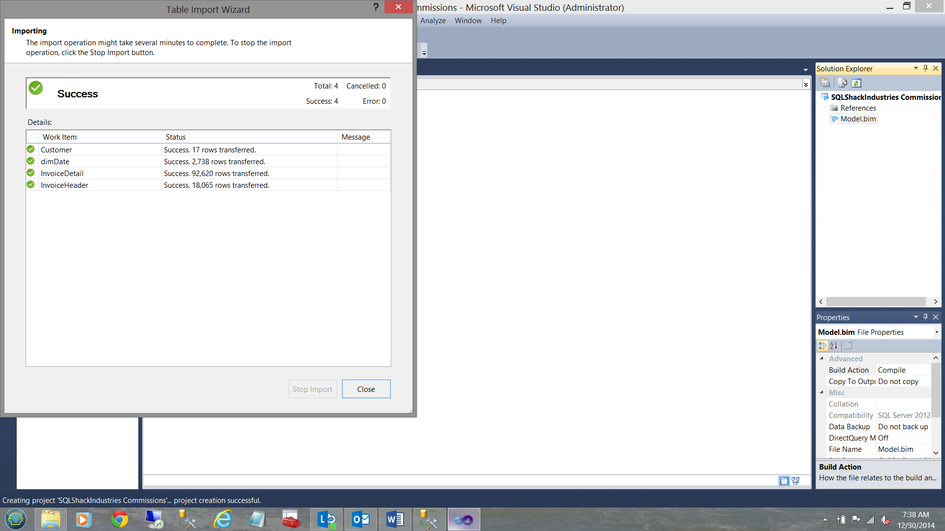
When the load is complete, we receive a “Success” notification (see above). Click “Close”.

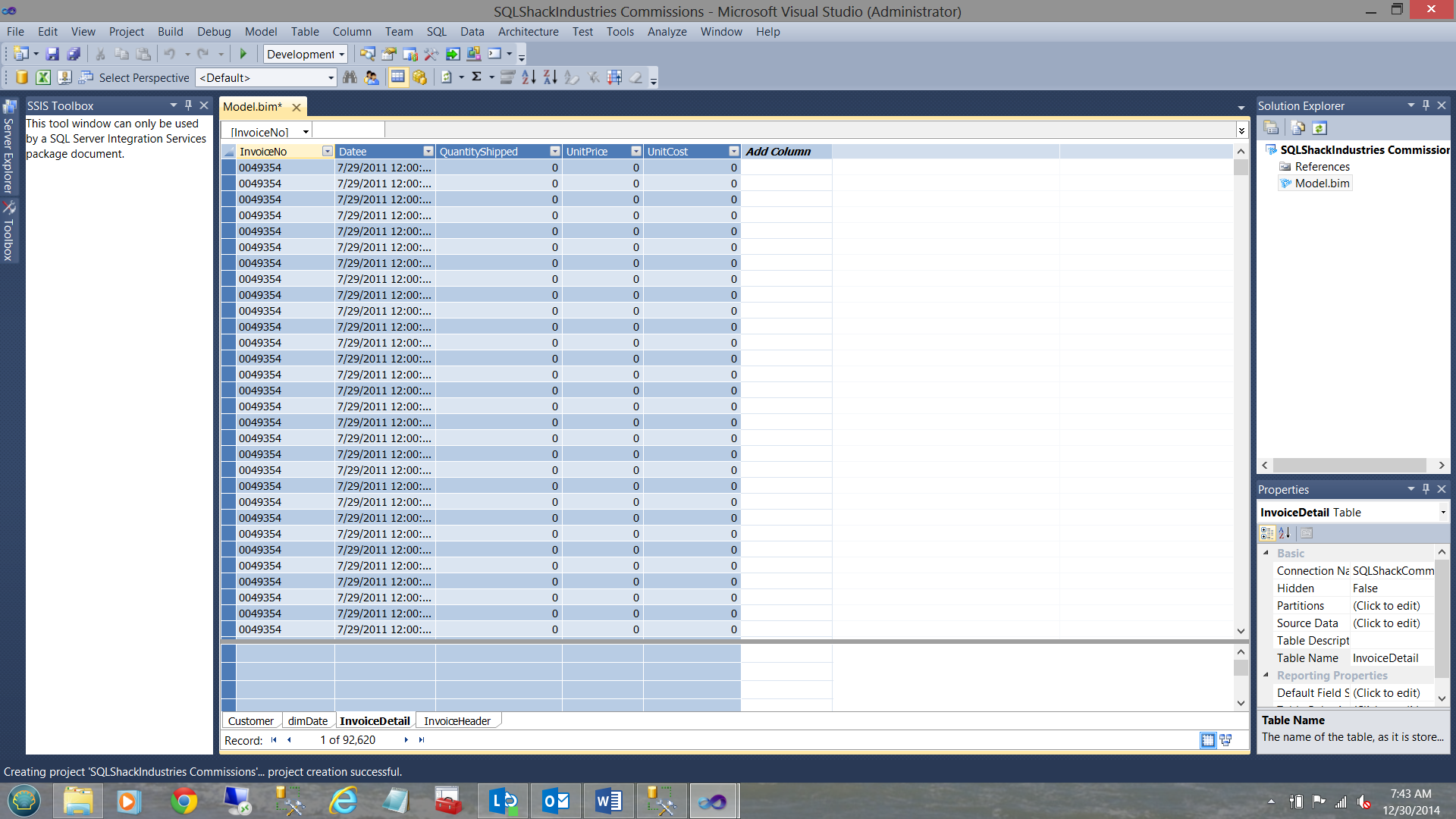
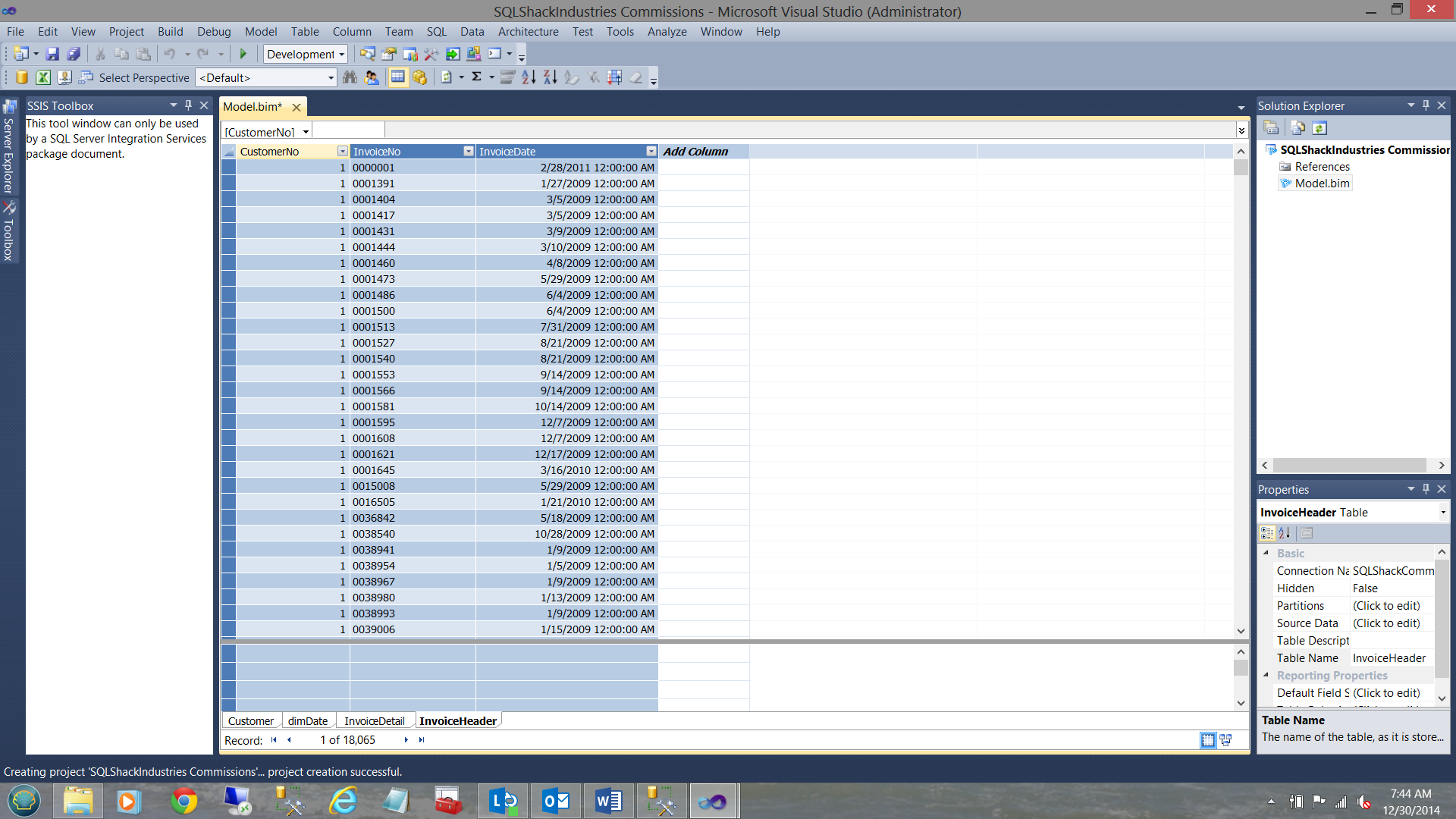
Our Imported Data

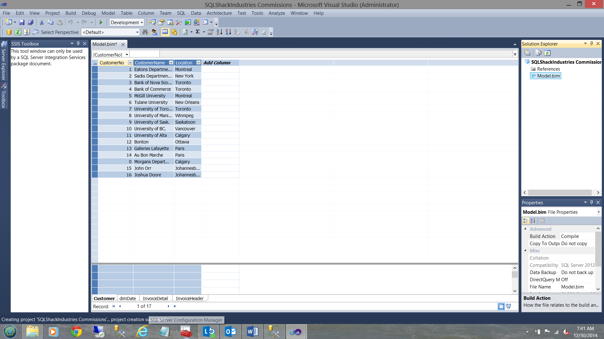
Making sense of this all

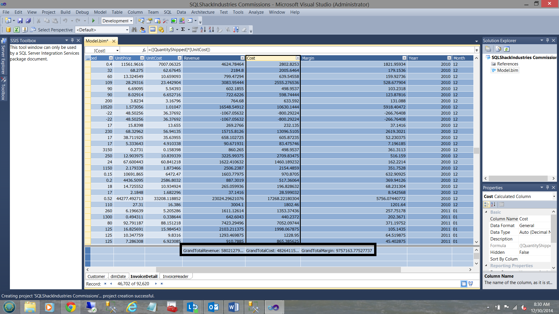
Whilst the necessary core data (for our exercise) is present, there are a few calculated fields that we wish to add to our “Invoice Detail” table. This table contains all of the items that SQLShack Industries have sold.

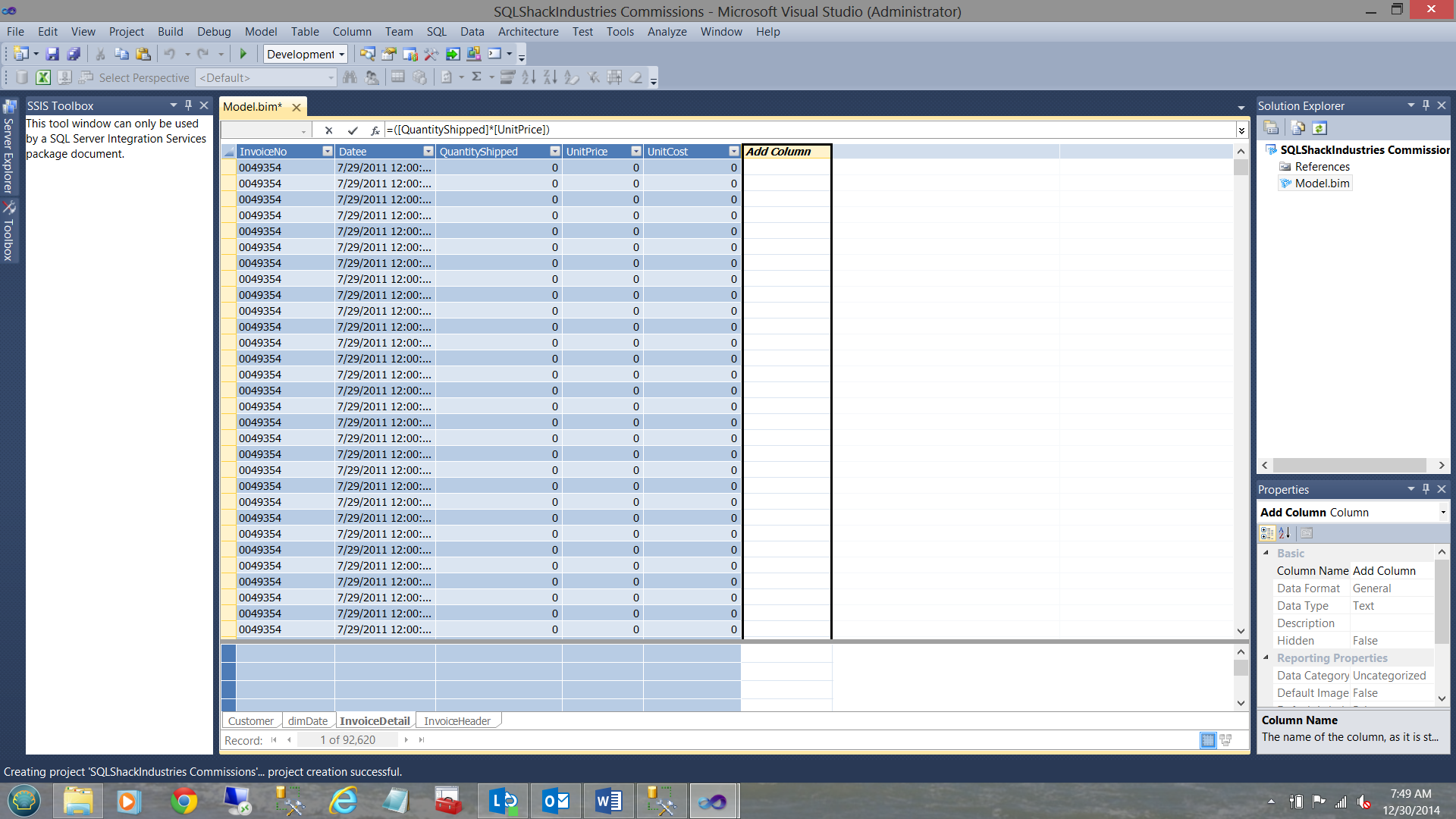
In the screen shot above we are going to create an additional column which we shall call “Revenue”. It is defined as “=([QuantityShipped]*[UnitPrice])” Not one’s typical way of creating a SQL expression and rightly so. Being within a tabular model, expressions must be programmed in DAX.

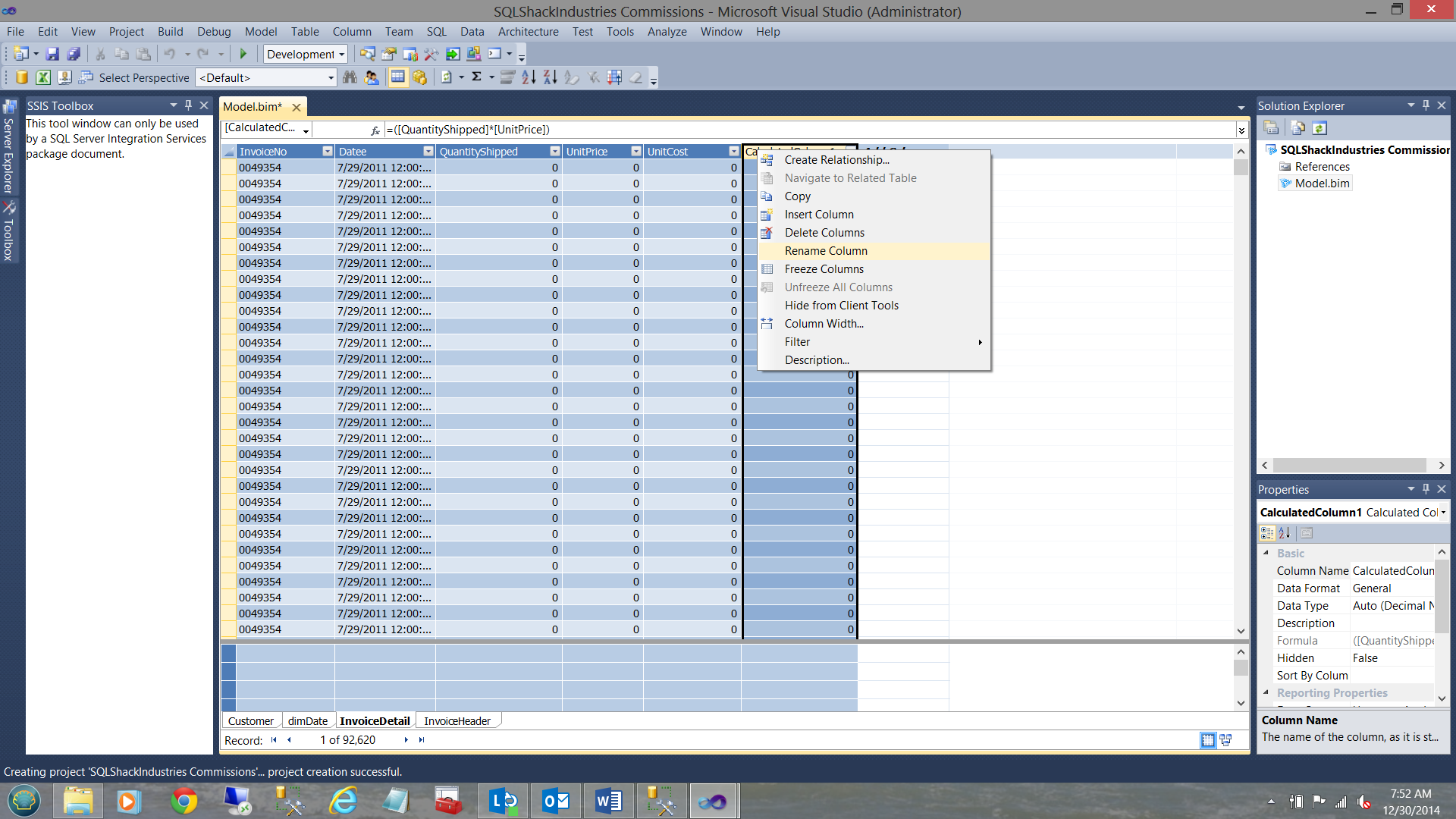
We rename our column “Revenue”.

In a similar manner we create

• “Cost”    =([QuantityShipped]*[UnitPrice])
• “Margin”  =([QuantityShipped]*[UnitPrice]) -([QuantityShipped] *[UnitCost])
• “Yearr”  =Year([datee])
• “Month”  =Switch(MONTH([datee]), 1, “01”, 2, “02”, 3, “03”, 4, “04”, 5, “05”, 6, “06”, 7, “07”, 8, “08”, 9, “09”, 10, “10”, 11, “11”, 12, “12”, “Unknown month number” )
• “Quarter” =Switch(MONTH([datee]), 1, “01”, 2, “01”, 3, “01”, 4, “02”, 5, “02”, 6, “02”, 7, “03”, 8, “03”, 9, “03”, 10, “04”, 11, “04”, 12, “04”, “Unknown Quarter” )

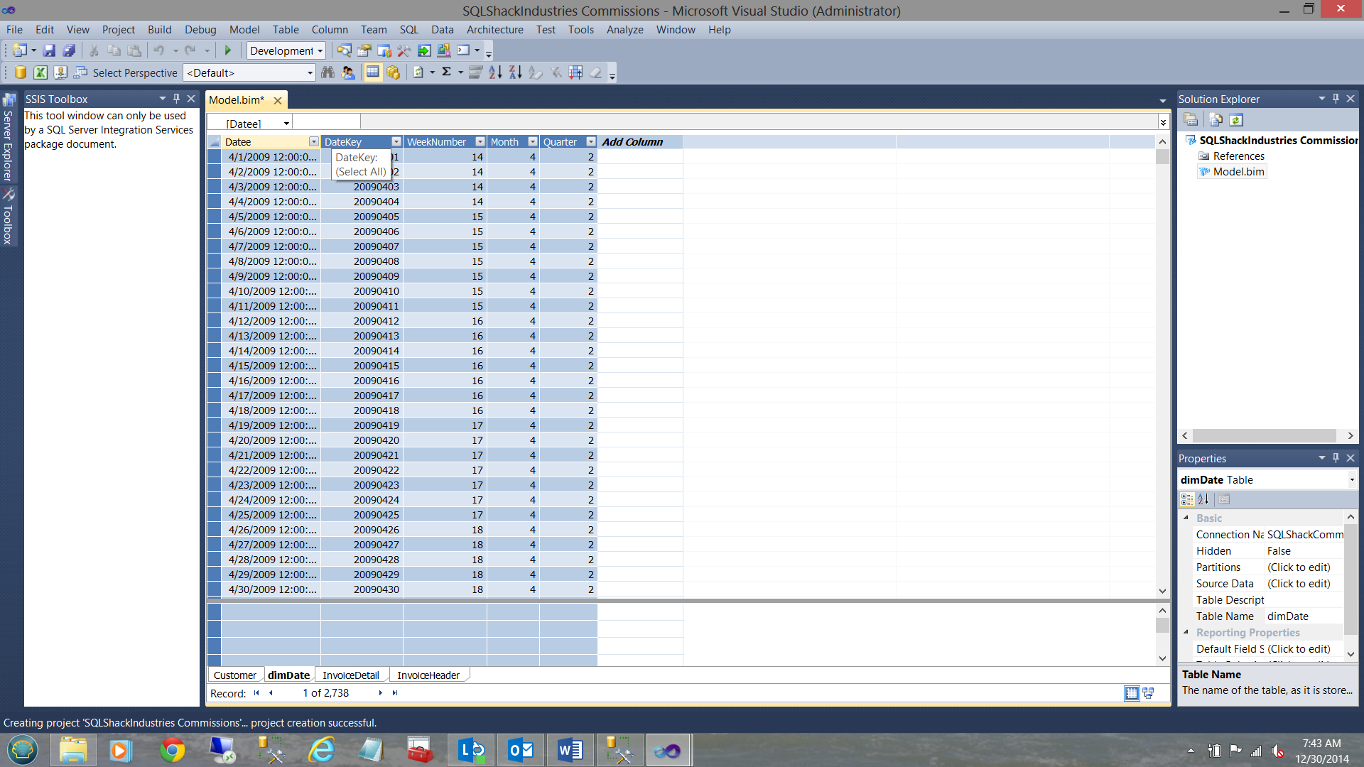
The results of these calculations may be seen above.

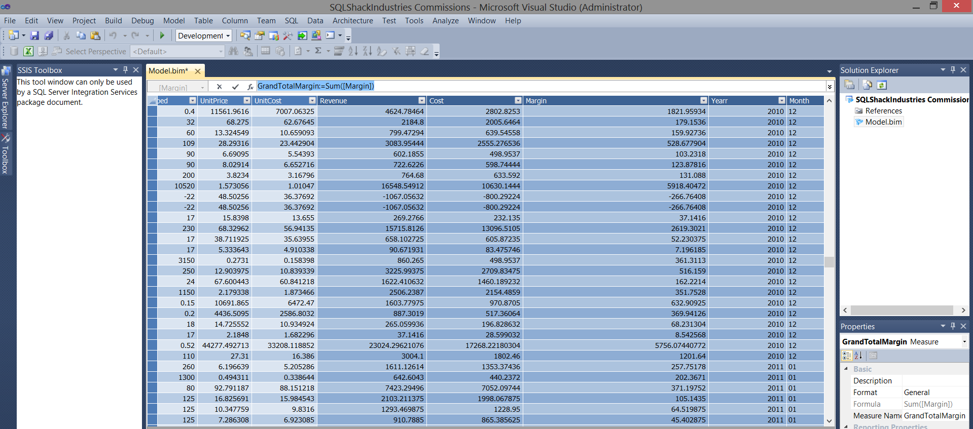
Creating our measures

Measures are “columns” or “summations” of varied field that are normally numeric. Example of this are “Sales figures for the month of December”.
We are going to create three measures “GrandTotal Revenue”, “GrandTotal Cost” and “GrandTotal Margin” (see below).

In a similar fashion create

• GrandTotalRevenue:=Sum([Revenue])
• GrandTotalCost:=sum([Cost])
• GrandTotalMargin:=Sum([Margin])

Switching to “Relational view” we find our four tables. We create the appropriate links as shown below:

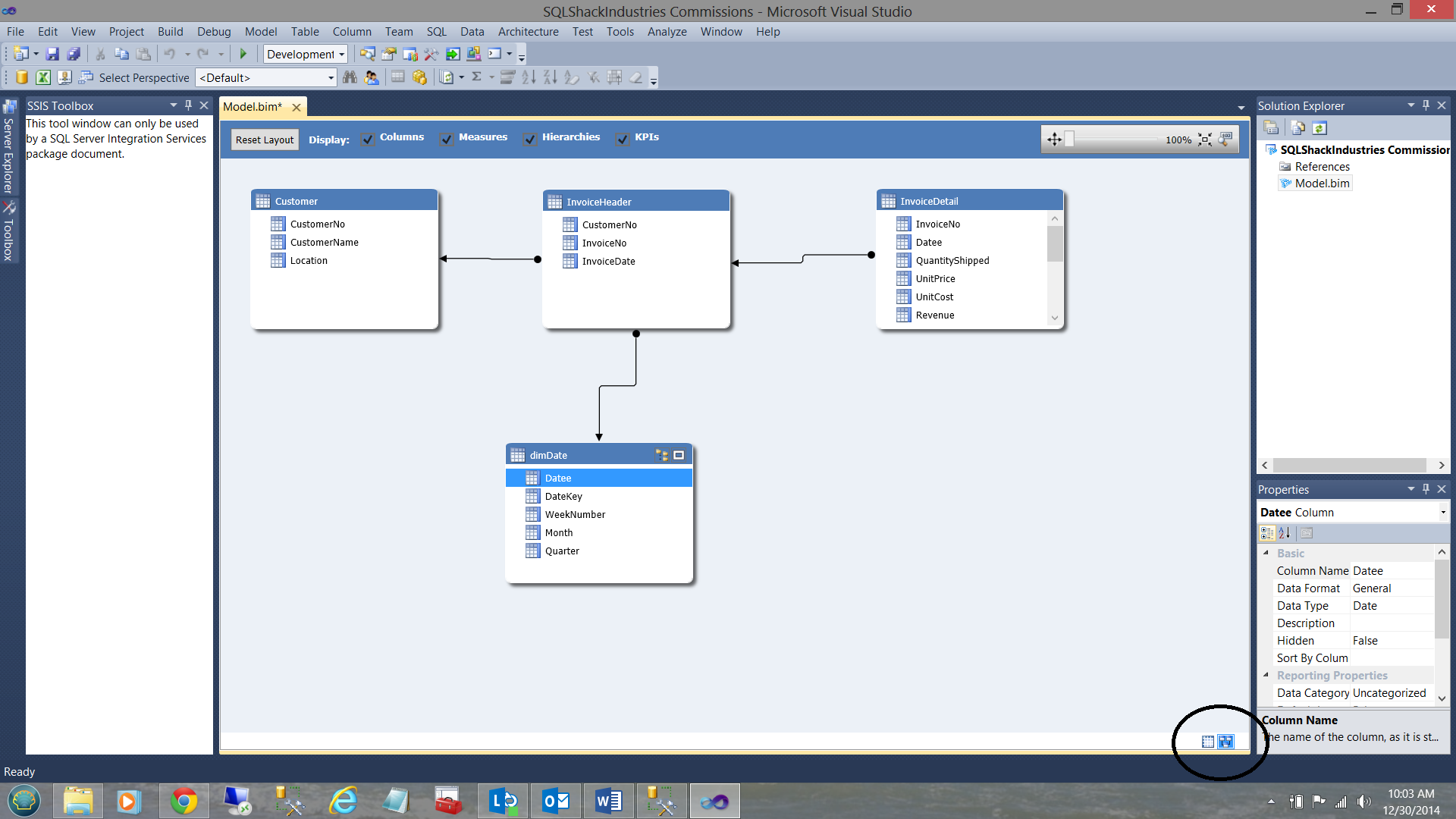
Having defined the “inner joins” between our tables, we are now in a position to deploy our model.

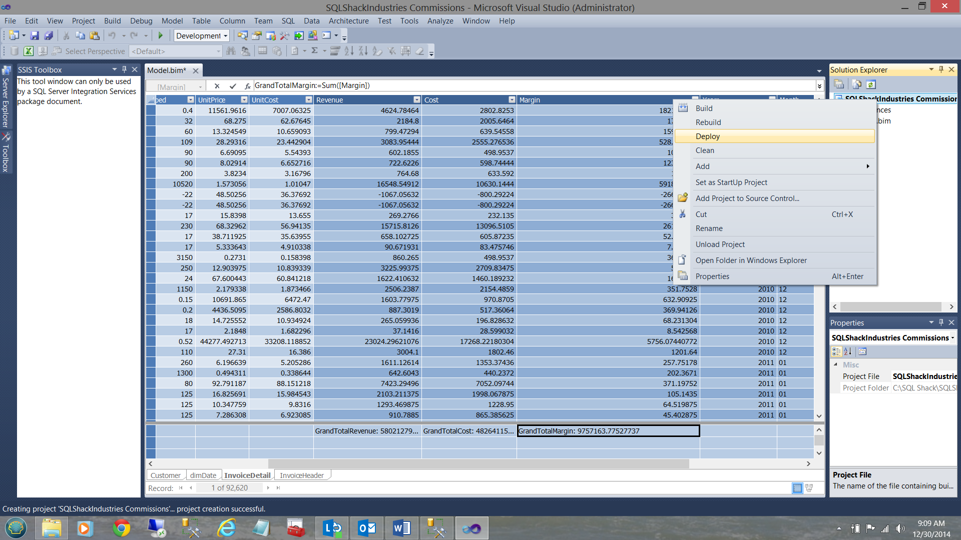
We choose “Deploy”

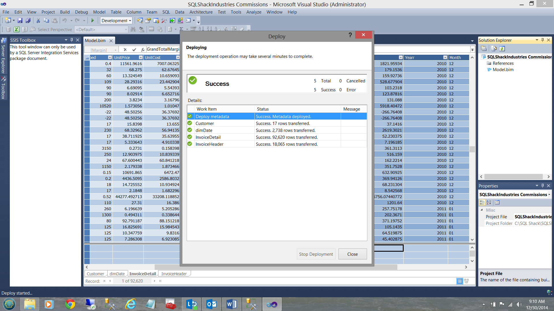
When deployment is complete we receive a “Success” notification and close out of SQL Server Data Tools.

Meanwhile back in SQL Server Management Studio

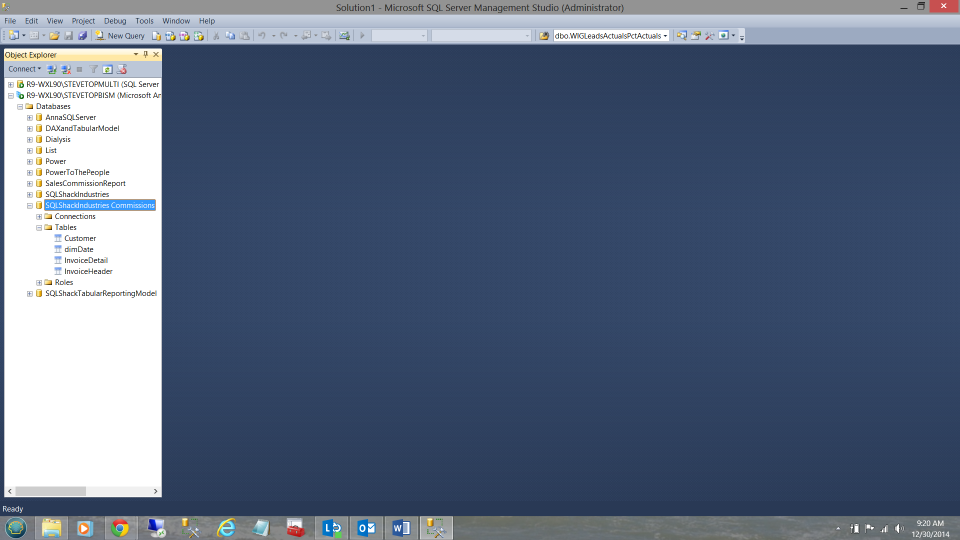
We note that our Analysis Services database has been created (see above).

Now to the “meat of the burger”

Now that we have our Analysis Services database, we are going to create a suite of informative reports.

Our first report will be our “Sales Commission Report”.

Opening SQL Server Data Tools once again, we create a new Reporting Services project. Should you be unfamiliar with creating projects, creating data source connections and datasets (within SQL Server Reporting Services), do have a look at my article entitled:

“Now you see it, now you don’t”
/now-see-now-dont/

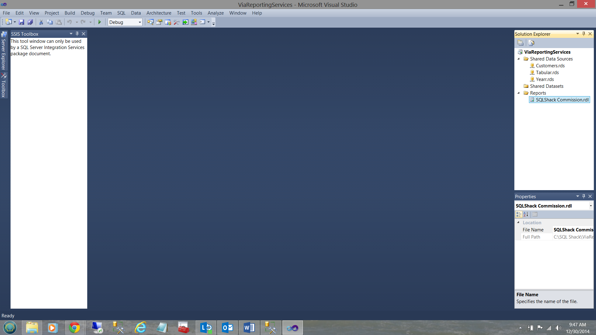
We first add a new report to the work surface. Our report will be called “SQLShack Commission” (see above). The differences between this report and reports that we have created in past are:

1. The data for this reports is coming from a Tabular Model.
2. A part of the requirement is to place the “Multi Select” option on for our report arguments.

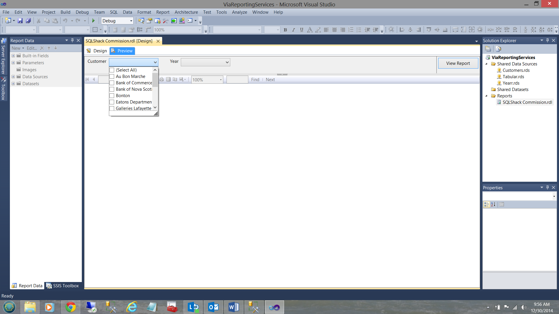
Multi-select on the customer name (see above)

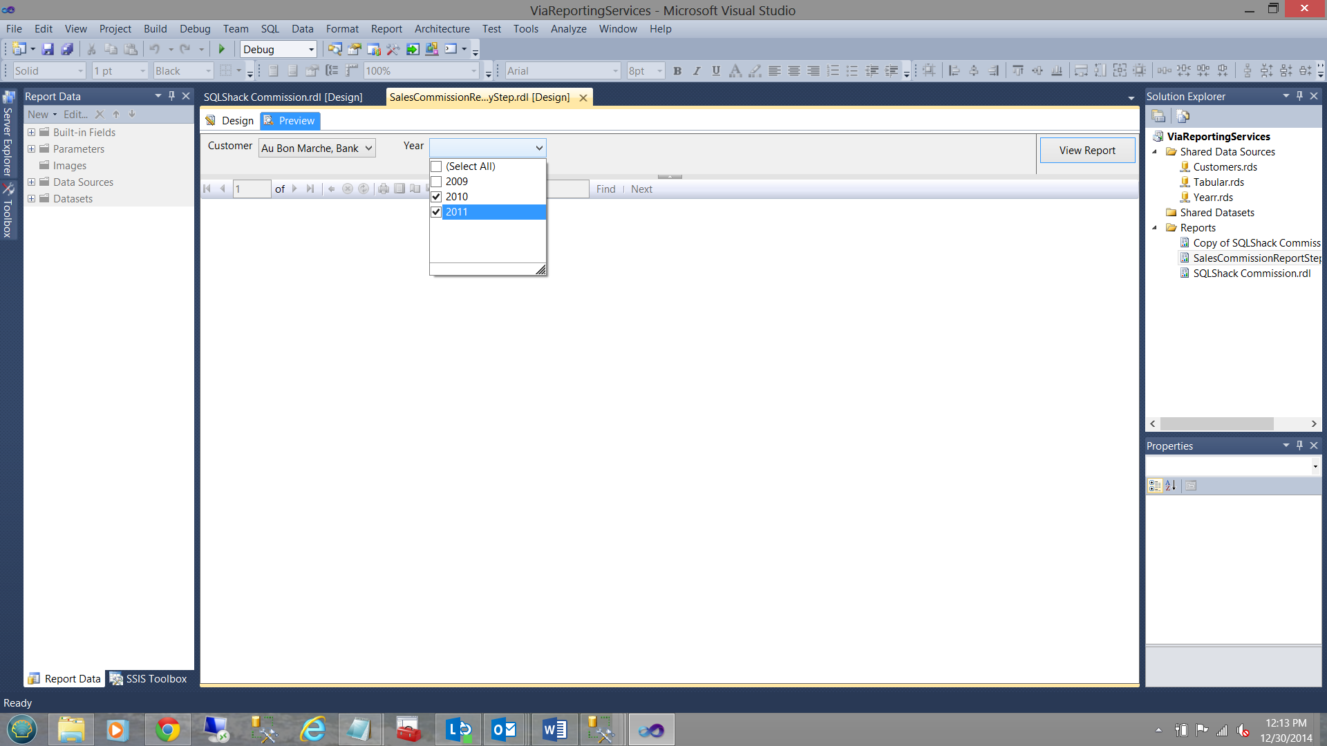
Multi-Select on the year (see below):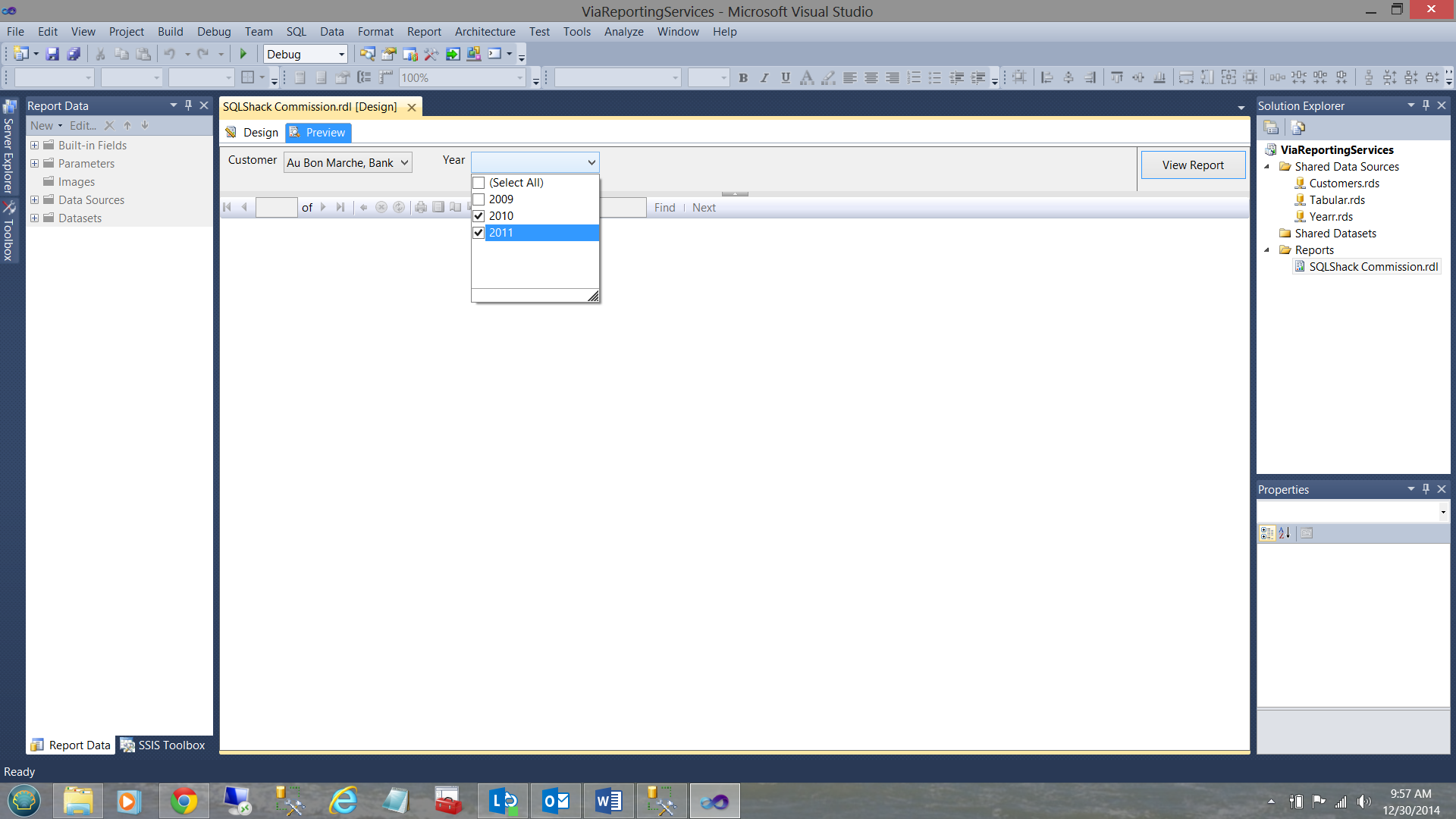

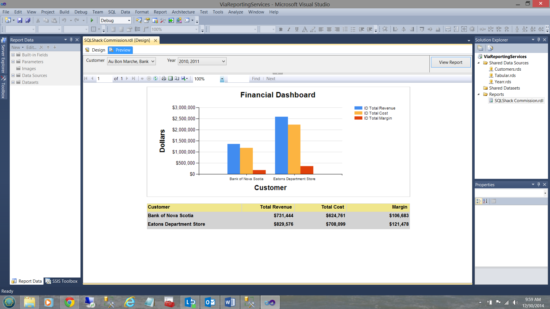
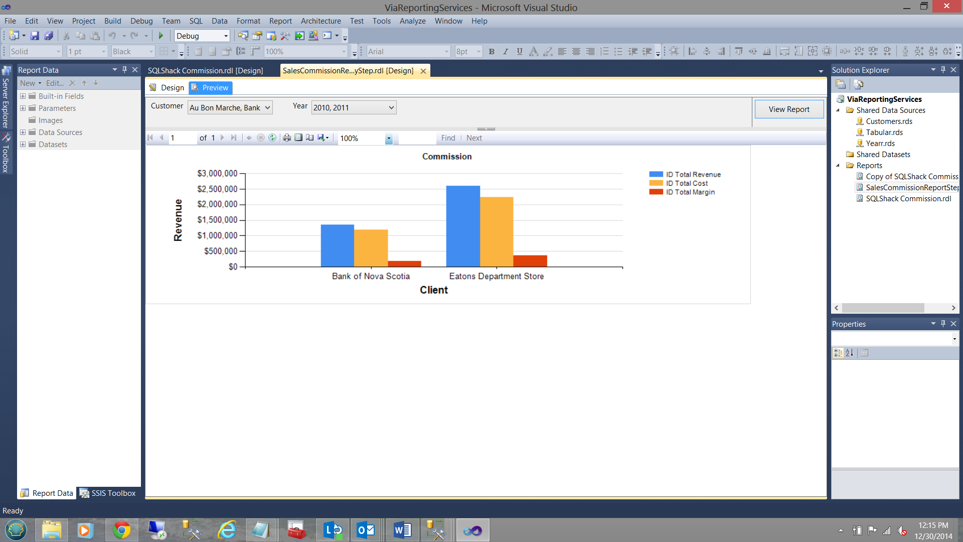
Our finished report will appear as follows:

How did we do that!!!

We begin by assembling a list of our current customers. This list may be created from relational data (which is what we shall do).

Using our relational data, we first create a new data source through to the customer table (see above). Having created our data source, we are now in a positon to create a new dataset which will hold the distinct customer names at run time.

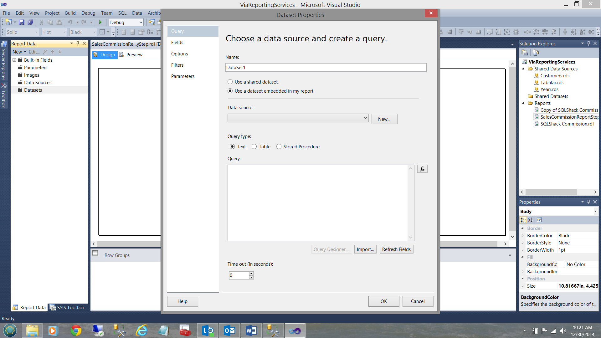
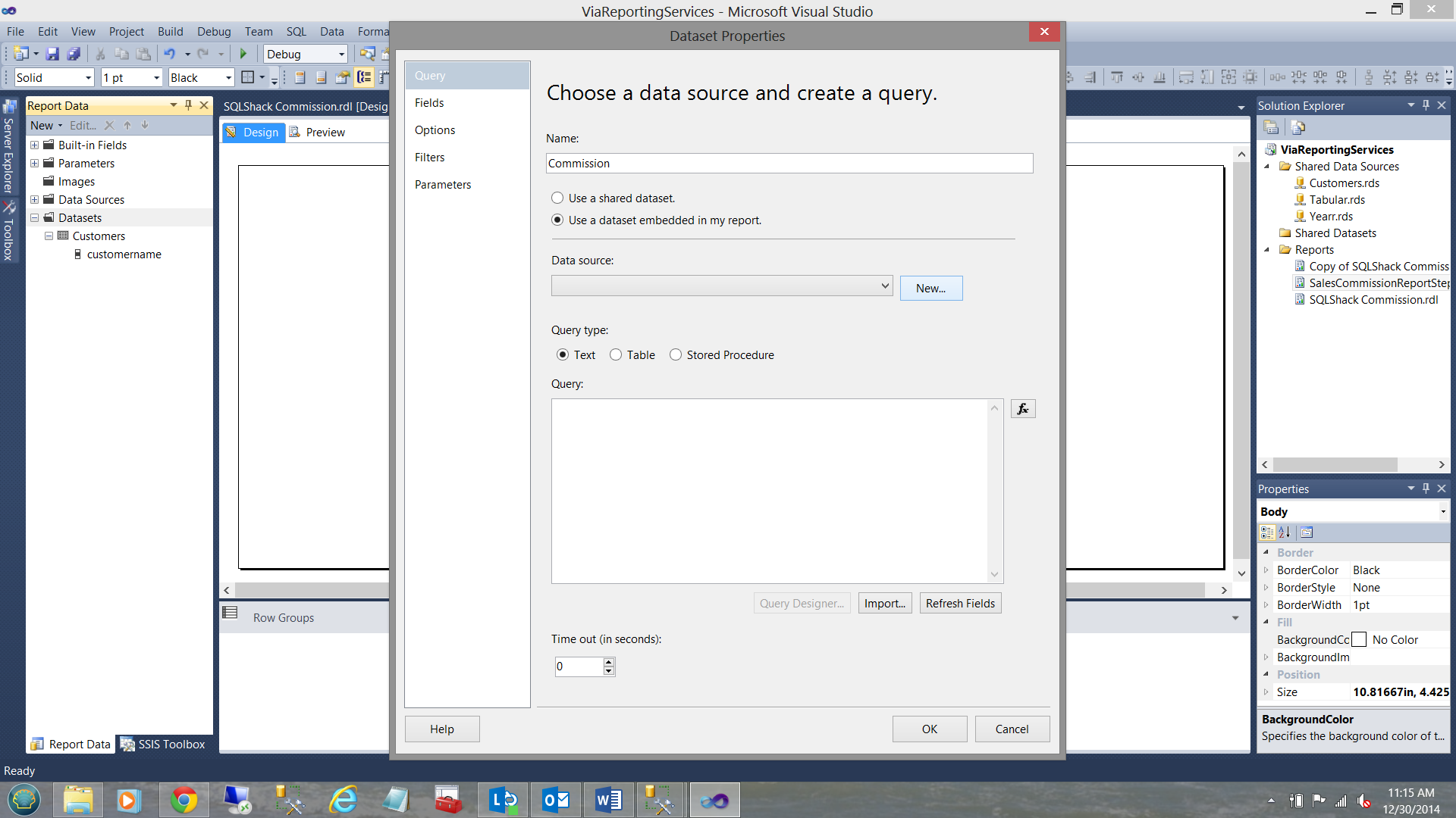
By right clicking on the Dataset folder, we add a new dataset (see below).

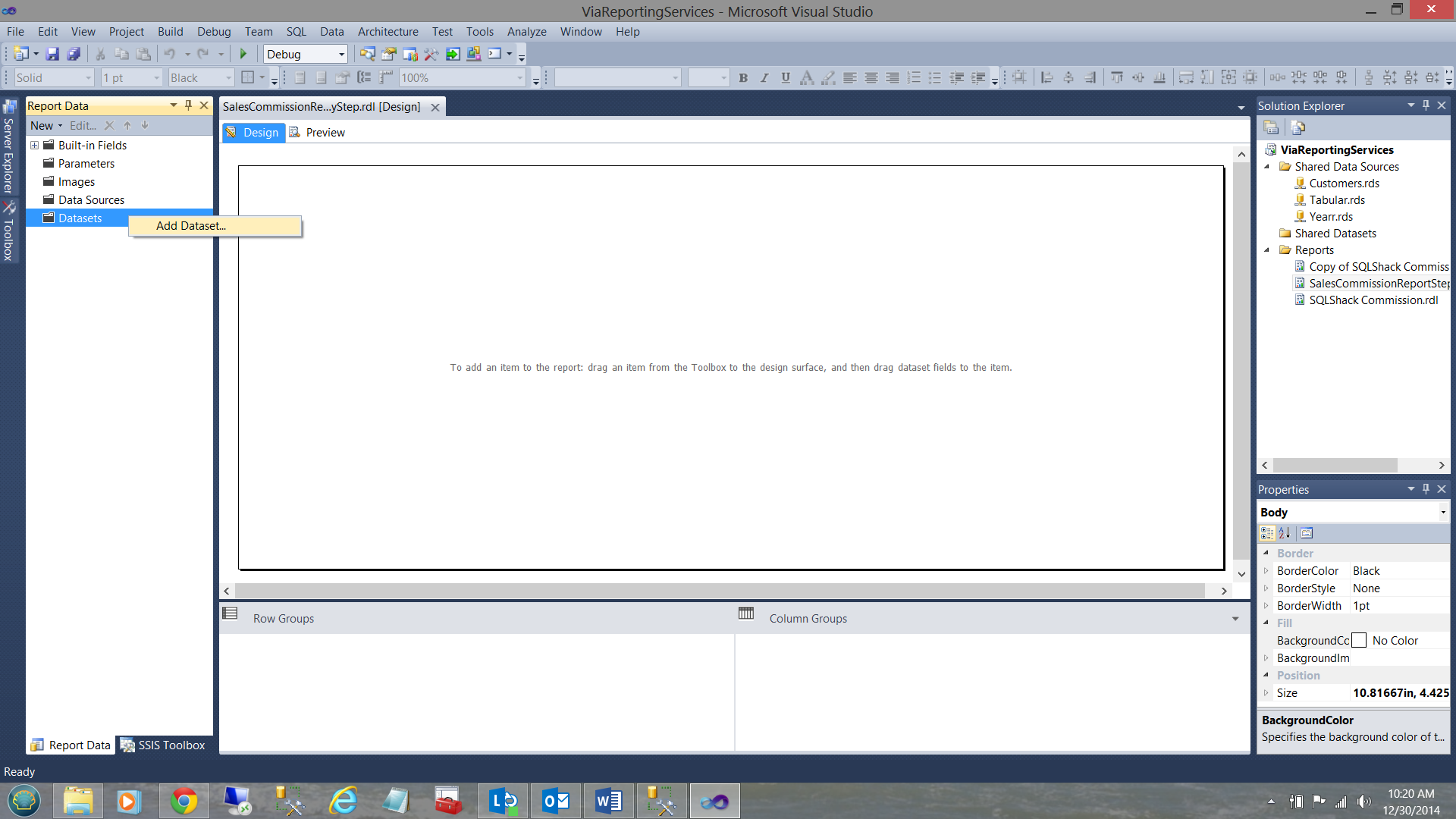
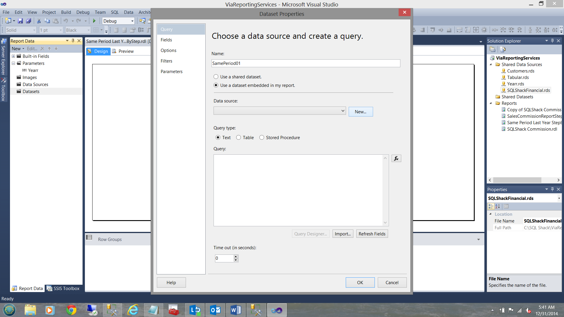
We choose an “embedded” dataset (see below).

Clicking the “New” button we shall create a new local data source so that this local data source will connect with the shared data source that we created above.

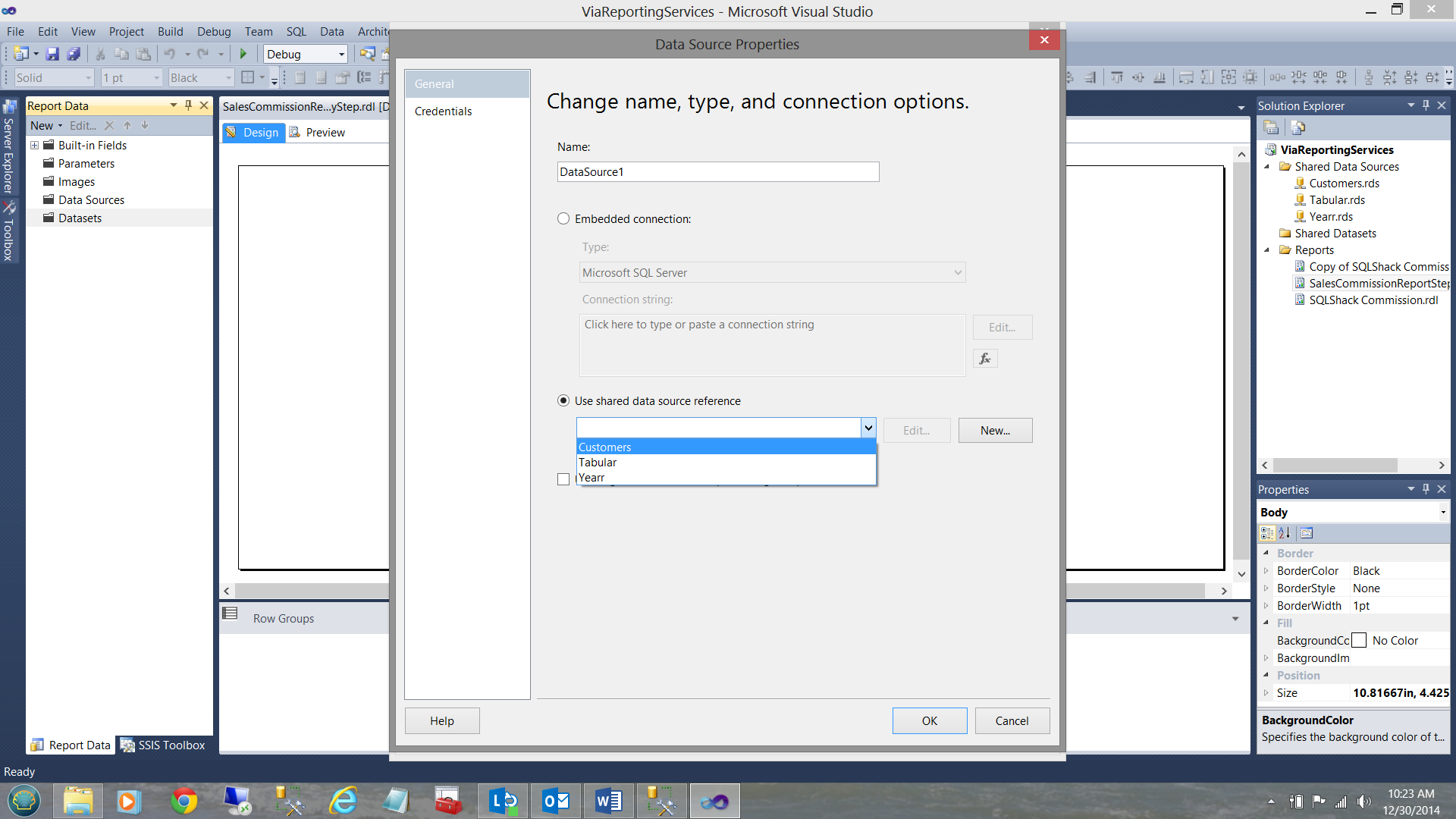
We click OK to complete the creation of the data source. All that remains is to define the contents of the dataset (see below).

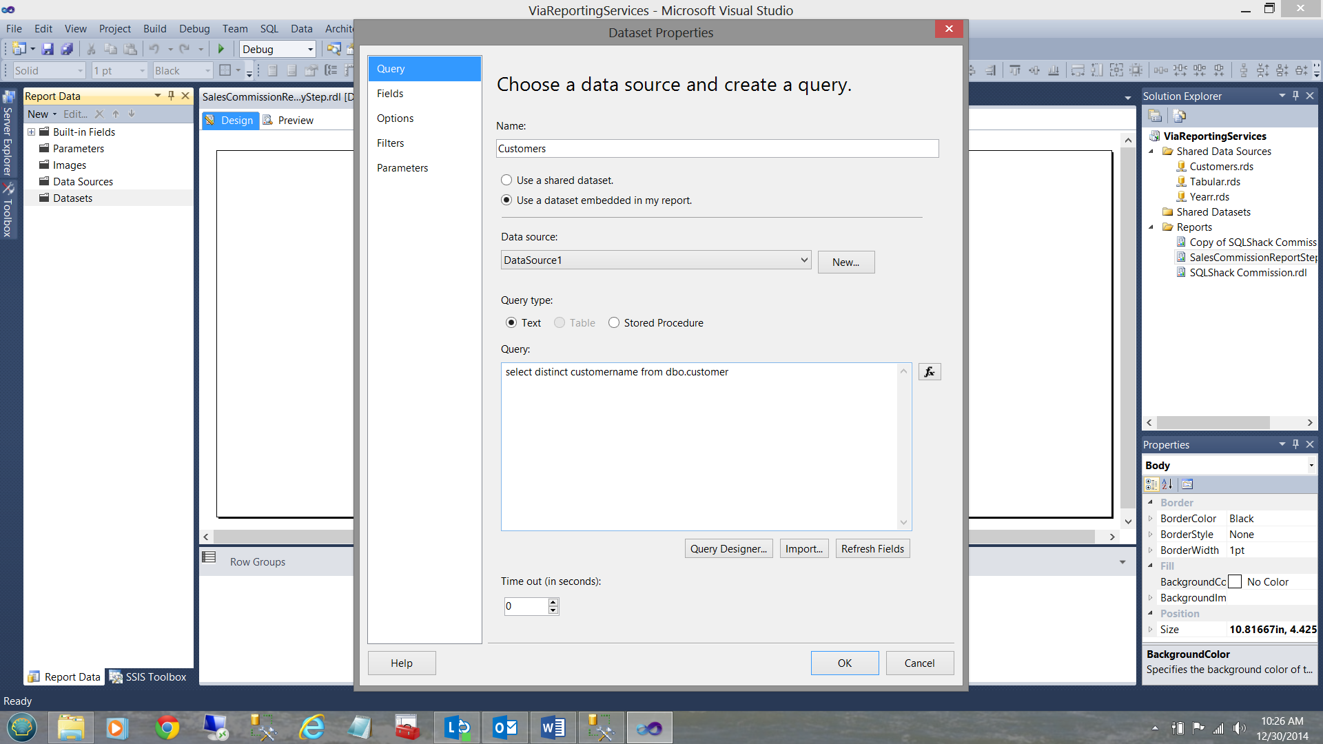
We place our query in the “Query” text box and the click “Refresh Fields” (see below).

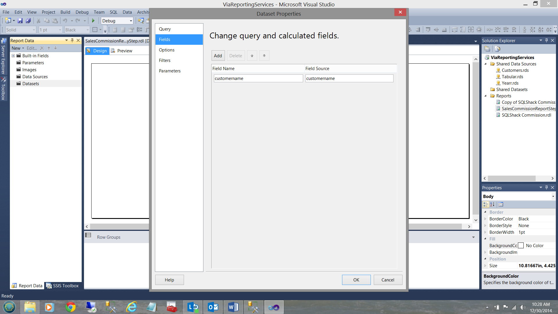
We click OK to complete the customer dataset.

Creating our parameters

Now that our customer dataset has been created, we must create two parameters. These two parameters will be utilized by the end user to set the desired customer(s) and the year(s) for which the user wishes to view the data.

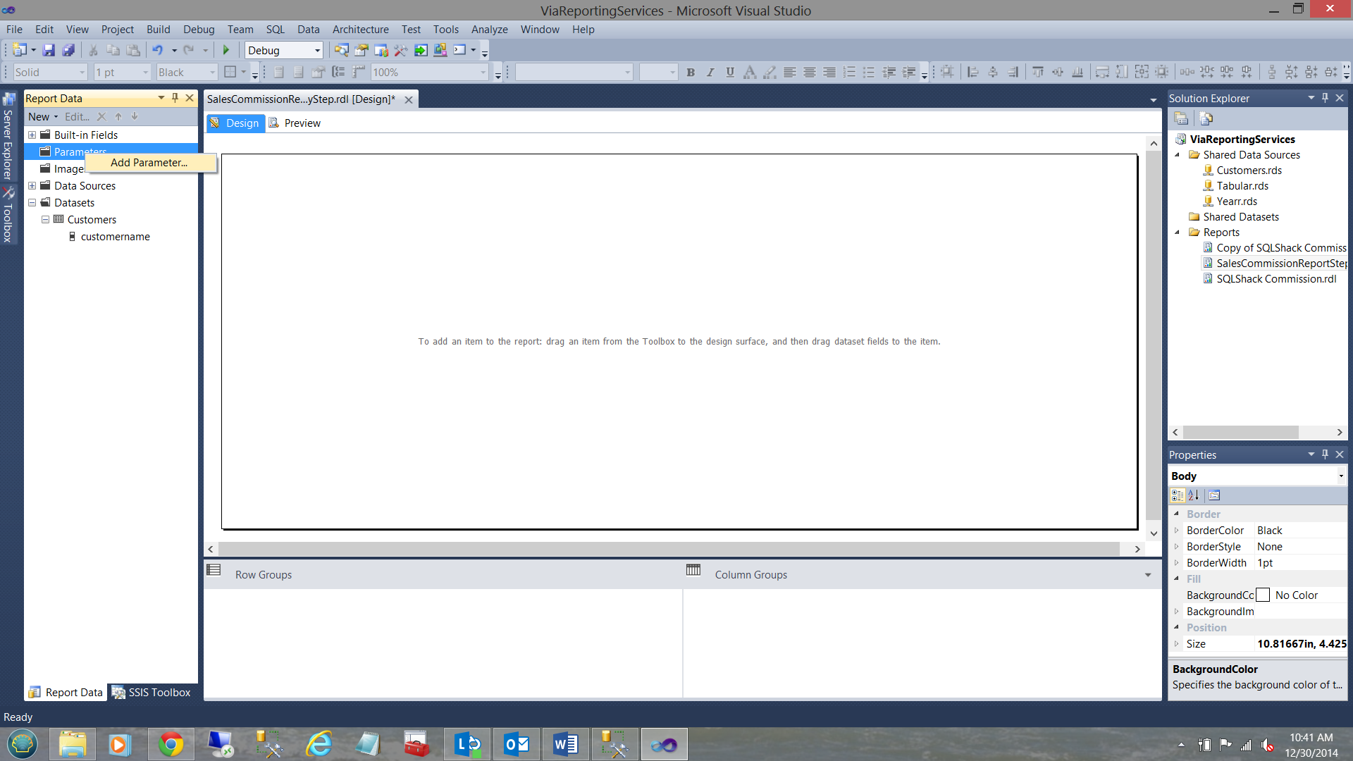
We right click on the “Parameters” folder and choose “Add Parameter”

Note above, that we have called the parameter “Customer” and that the prompt will be “Customer”. More importantly, note that we select the “Allow multiple values” option.

Moving on to the “Available Values” tab, we set the properties as follows (see below).

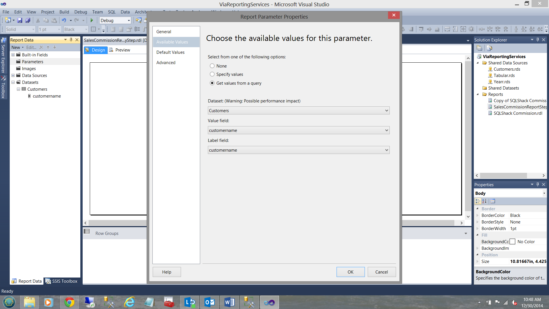
Note that we shall obtain our distinct names from the dataset that we created a few moments ago.

I click OK to exit the “Report Parameter Properties” window.
In a similar fashion, we create a “Yearr” parameter (see below).

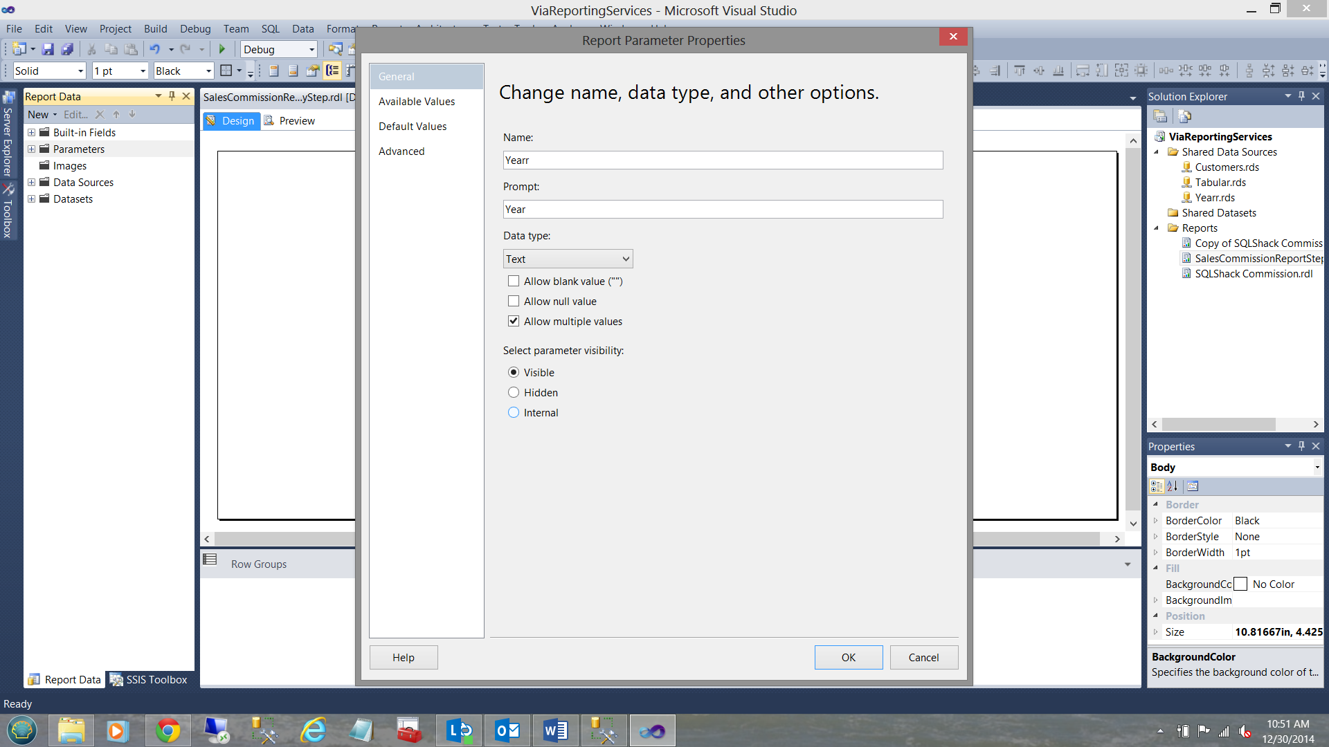
However in this case and for the sake of simplicity we shall “hard wire” our “Yearr” values (see below).

Having set up our parameters, we are now in a position to create the necessary code to extract the financial data for the customer(s) and the time period selected by the user.
The code for this may be seen below.

DAX code

The lines of code in yellow (see above) are the query predicate. It should be remembered that DAX is very similar to MDX code and Reporting Services accumulates the user selected arguments in comma delimited format which is NOT compatible to the DAX language.
What these lines of code are really saying is that we are looking for record(s) whose leaf level value(s) is / are one of our customer names that the user selected and for the year(s) selected.

All that you wanted to know about how to place the query into a Reporting Services dataset.

Believe it or not Microsoft has not got this one right yet and I raised the issue at the MVP conference last fall.

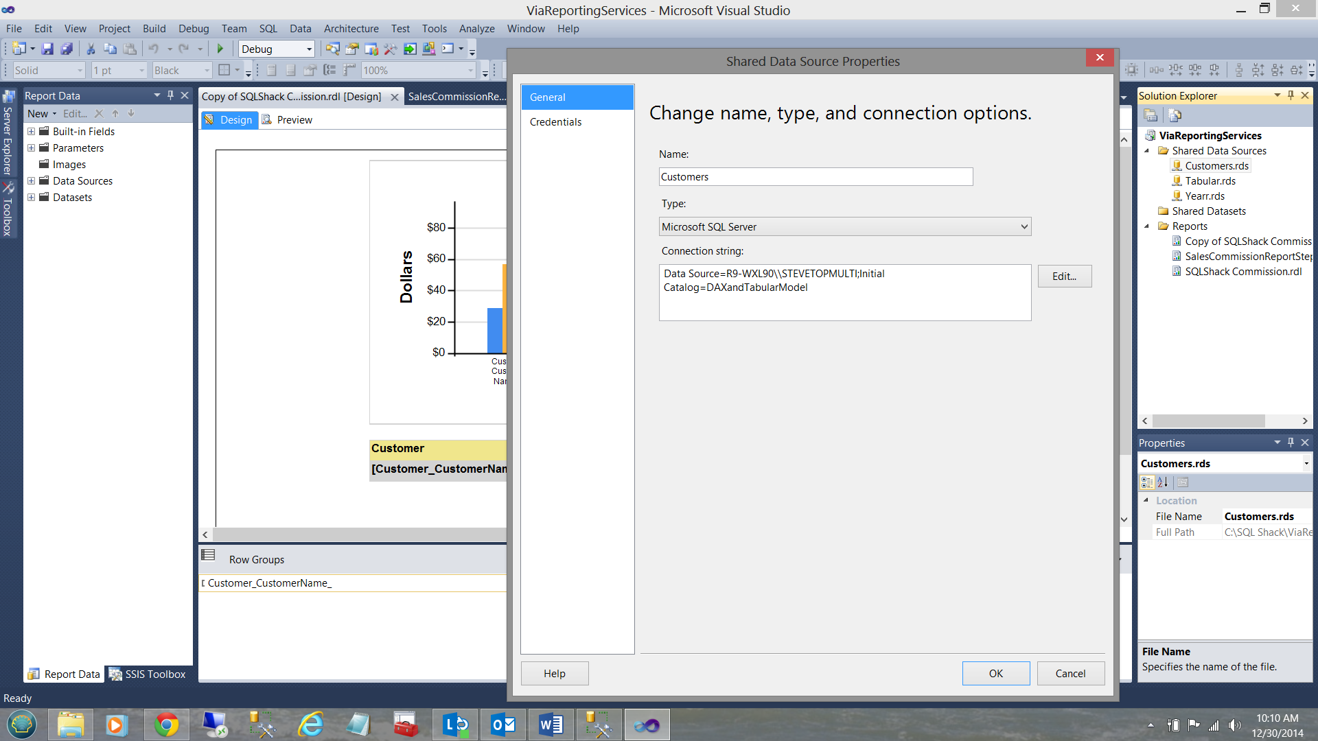
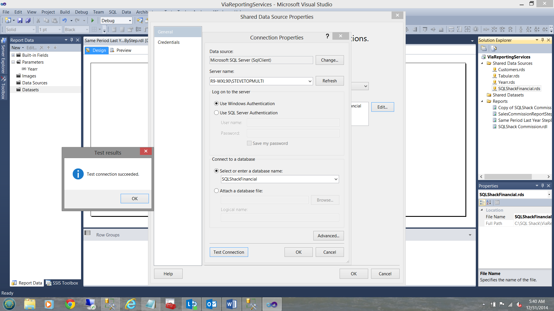
For this portion of the exercise, the data source is our Analysis Services database “SQLShackIndustries Commissions”.

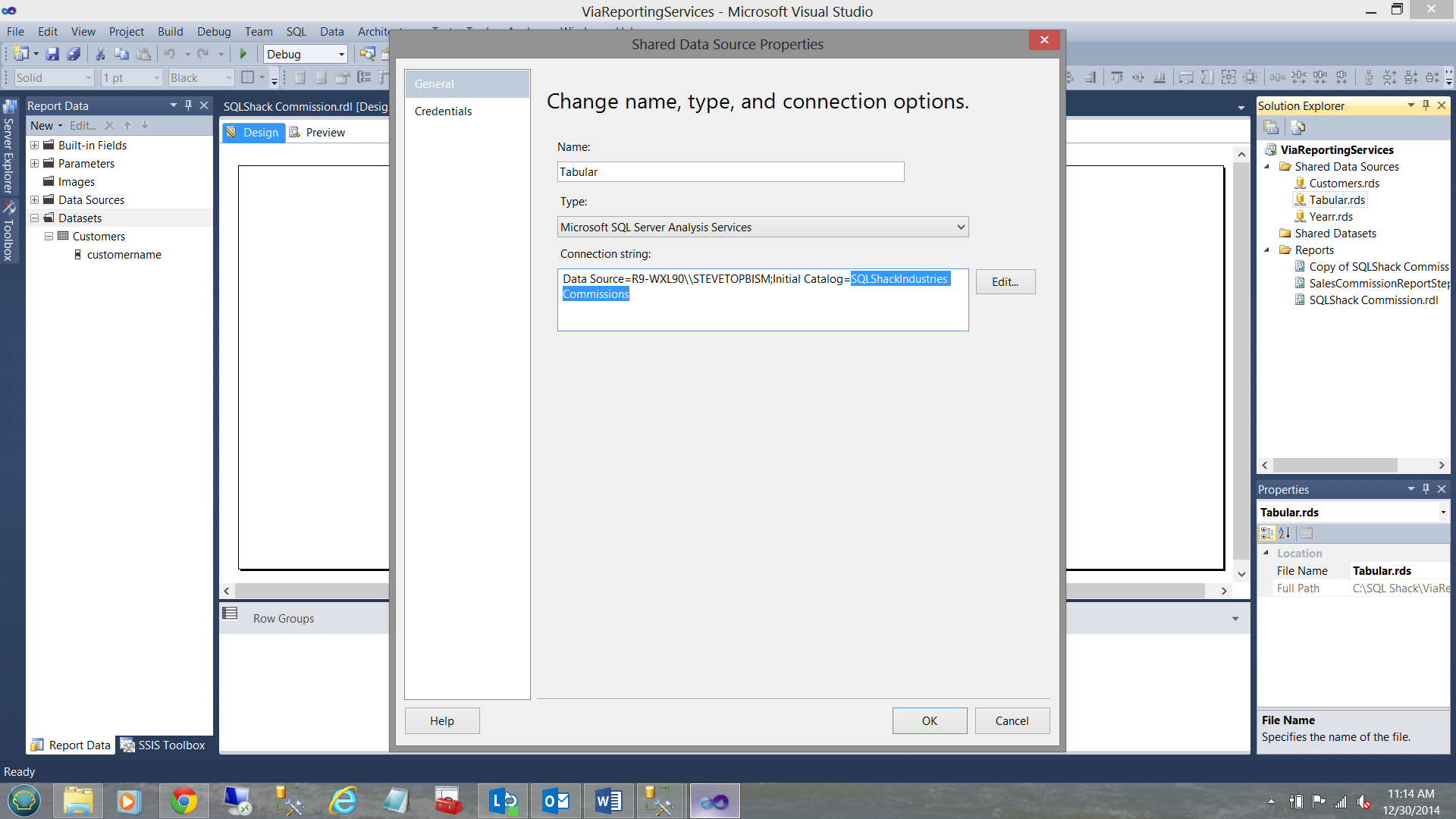
Our connection may be seen above.
The connection established, we now create a dataset to the hold the financial result set.

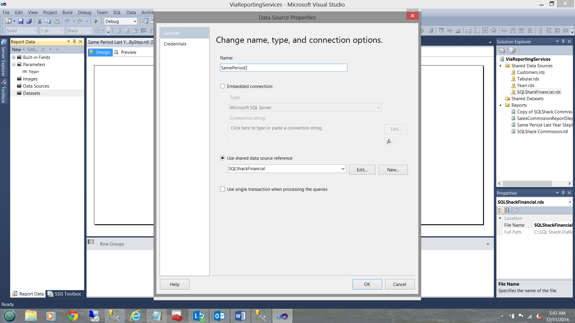
We opt for the “New” option for the local “Data source” as the location of the data is different to that of the customer data that we looked at a few minutes back.

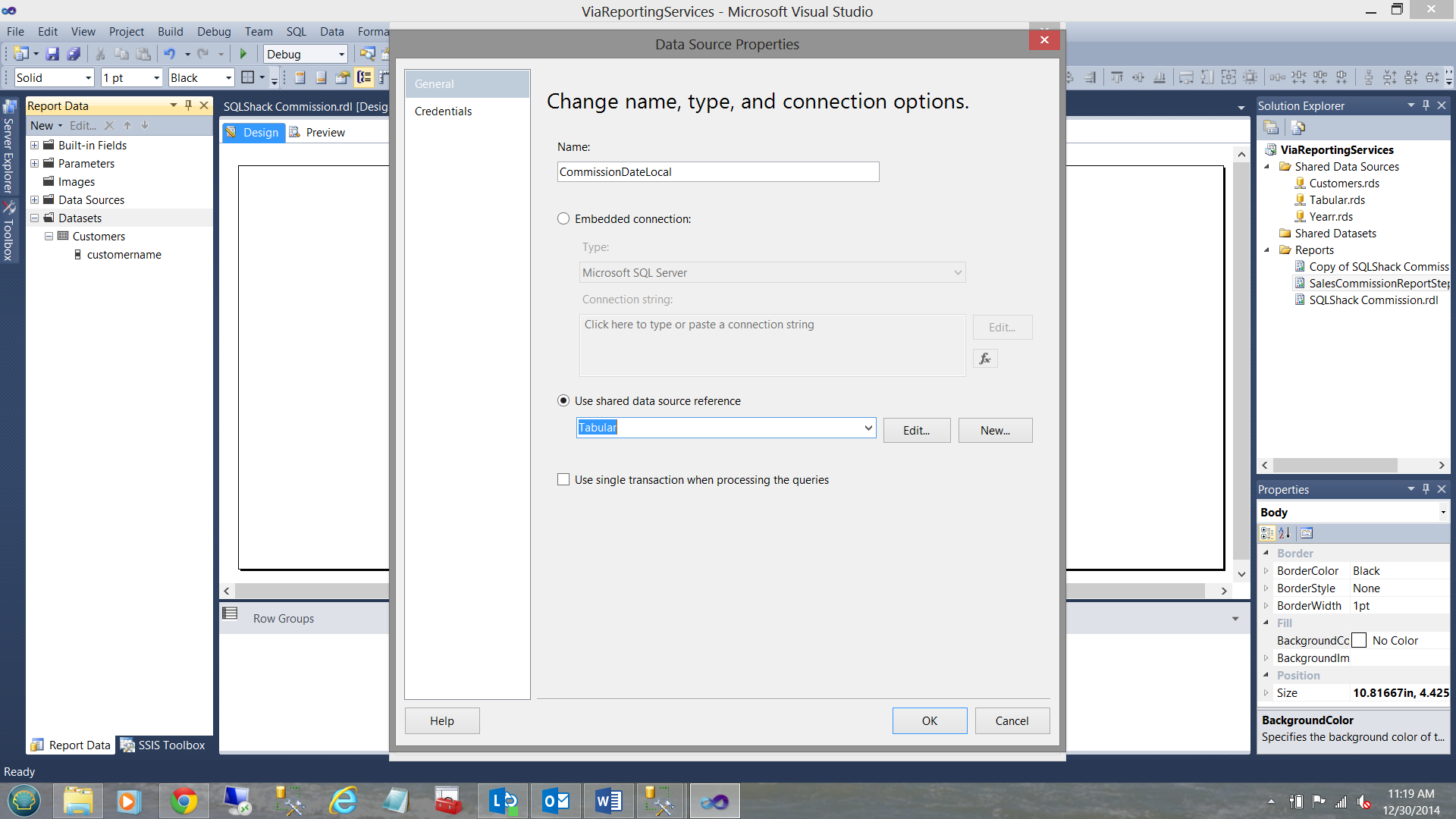
Note that we opt to utilize the “Use shared data source reference” Tabular. We click OK.

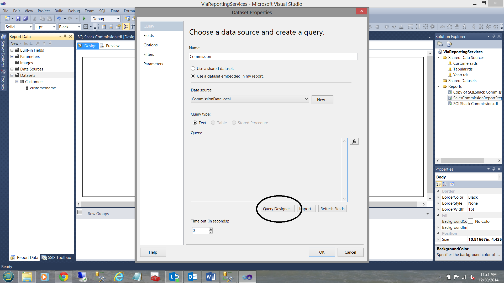
NOTE!!! .. the “Query” textbox is “Greyed” out and we CANNOT drop our code into that box which under normal circumstances (with relational queries) we would be able to do.

We MUST do a work around to place the code where it should be.

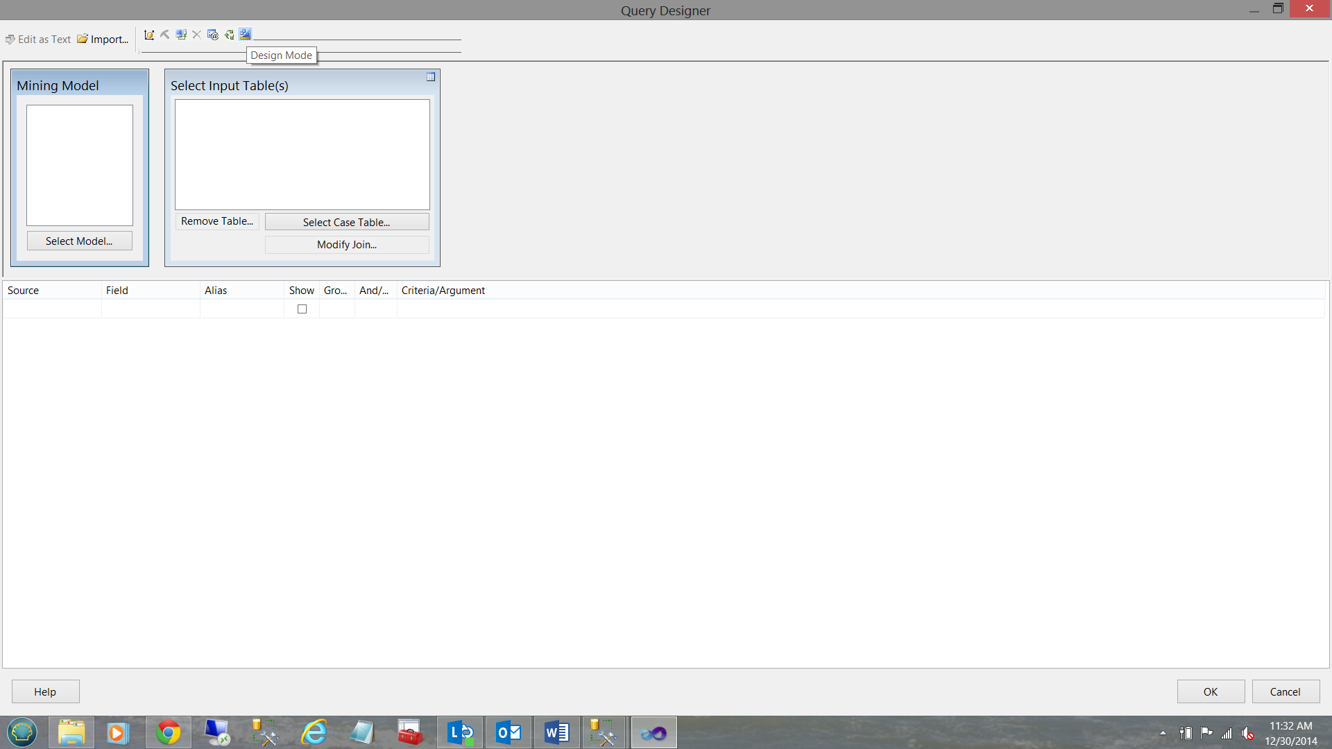
We click the “Query Designer” button (see above). The “Query Designer” opens.

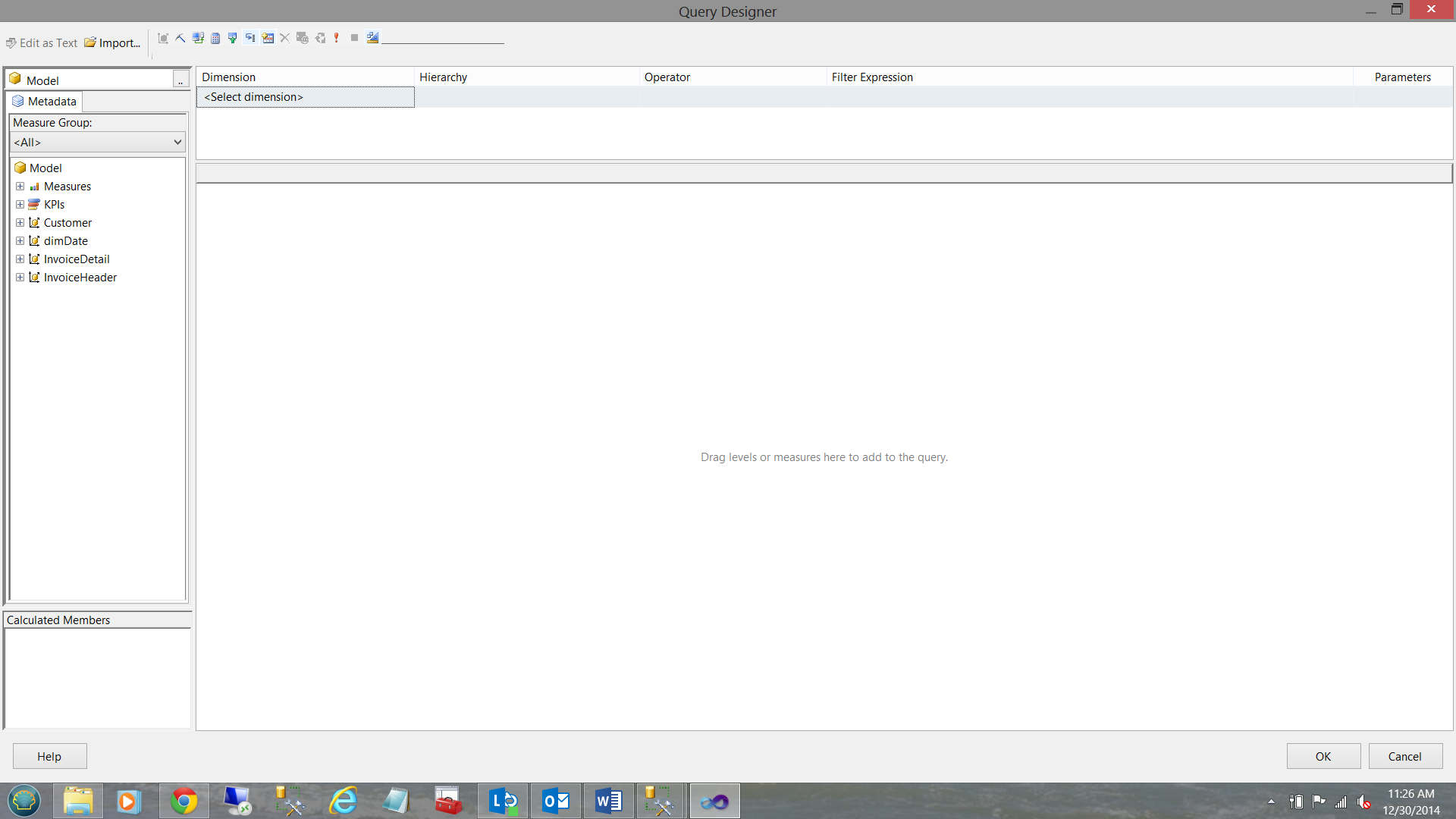
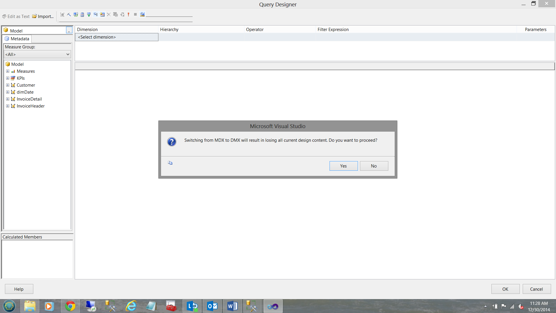
We select “Command Type DMX” for the top ribbon (see below)

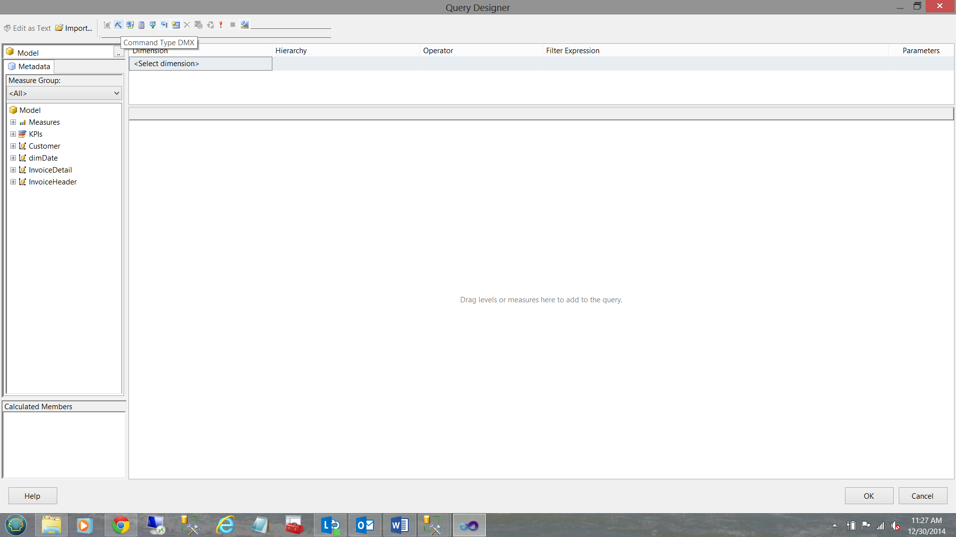
We received a warning to which we reply “Yes” (see below).

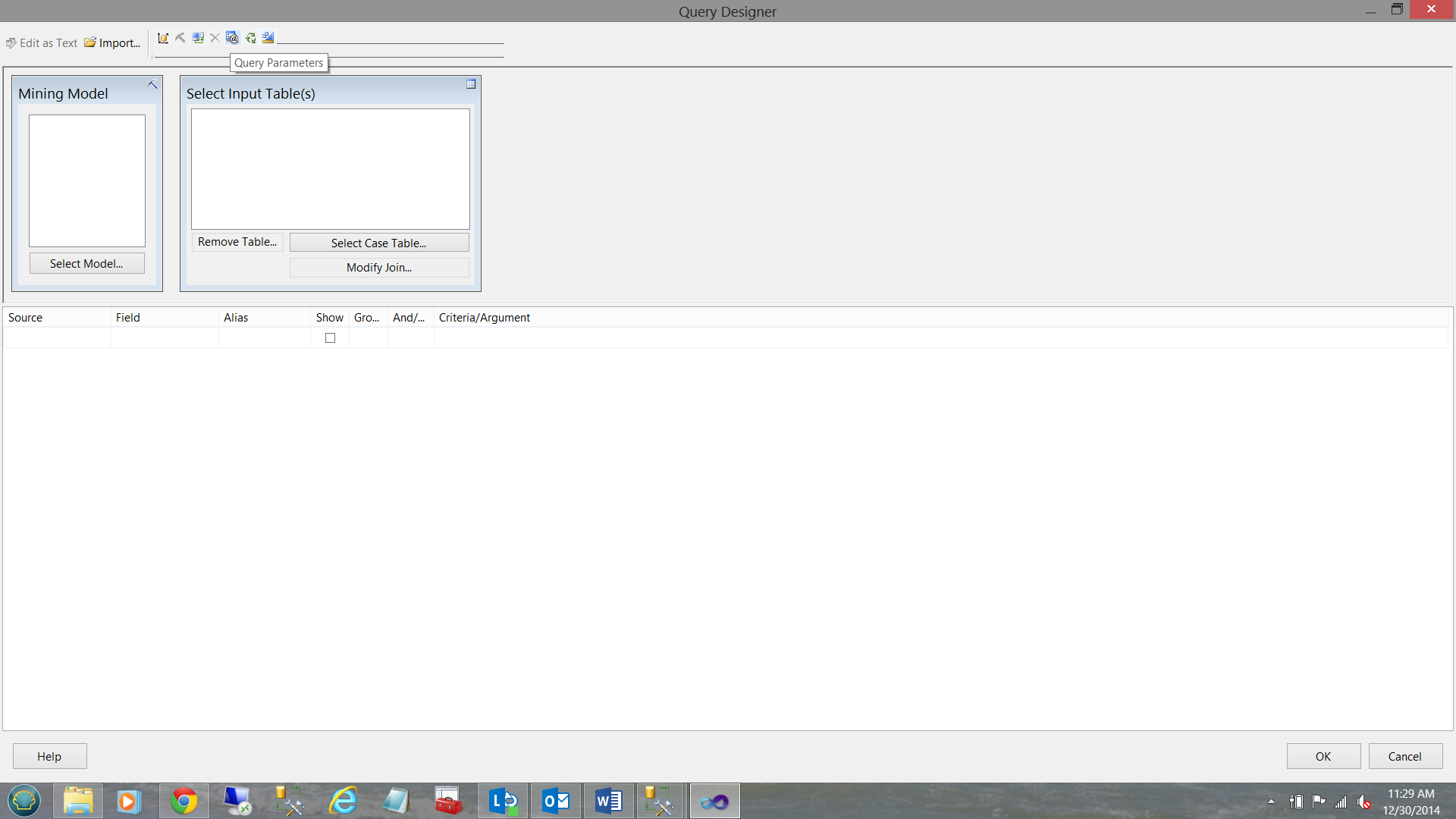
The DMX query window opens and we select the “Query Parameters” option from the ribbon on top (see below).

We code the parameters that will be required by our report (see below).

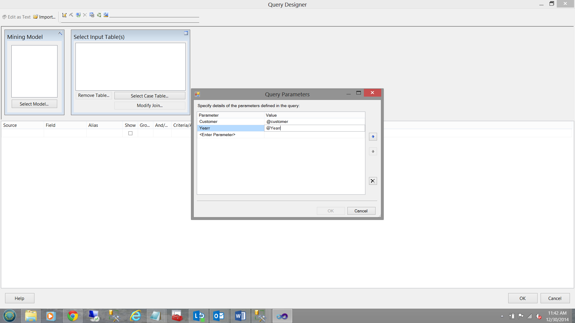
We click OK to accept the coding of the two parameters and we are returned to the design surface.

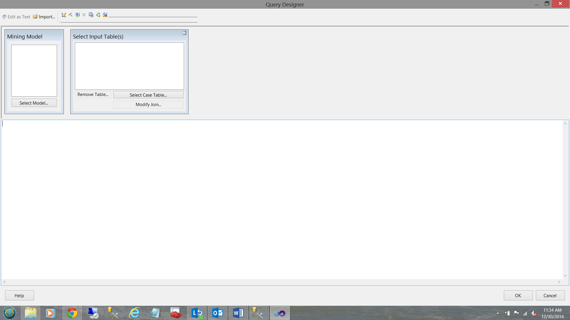
We now switch to “Design Mode” from the menu ribbon (see previous screenshot prior to the one above).

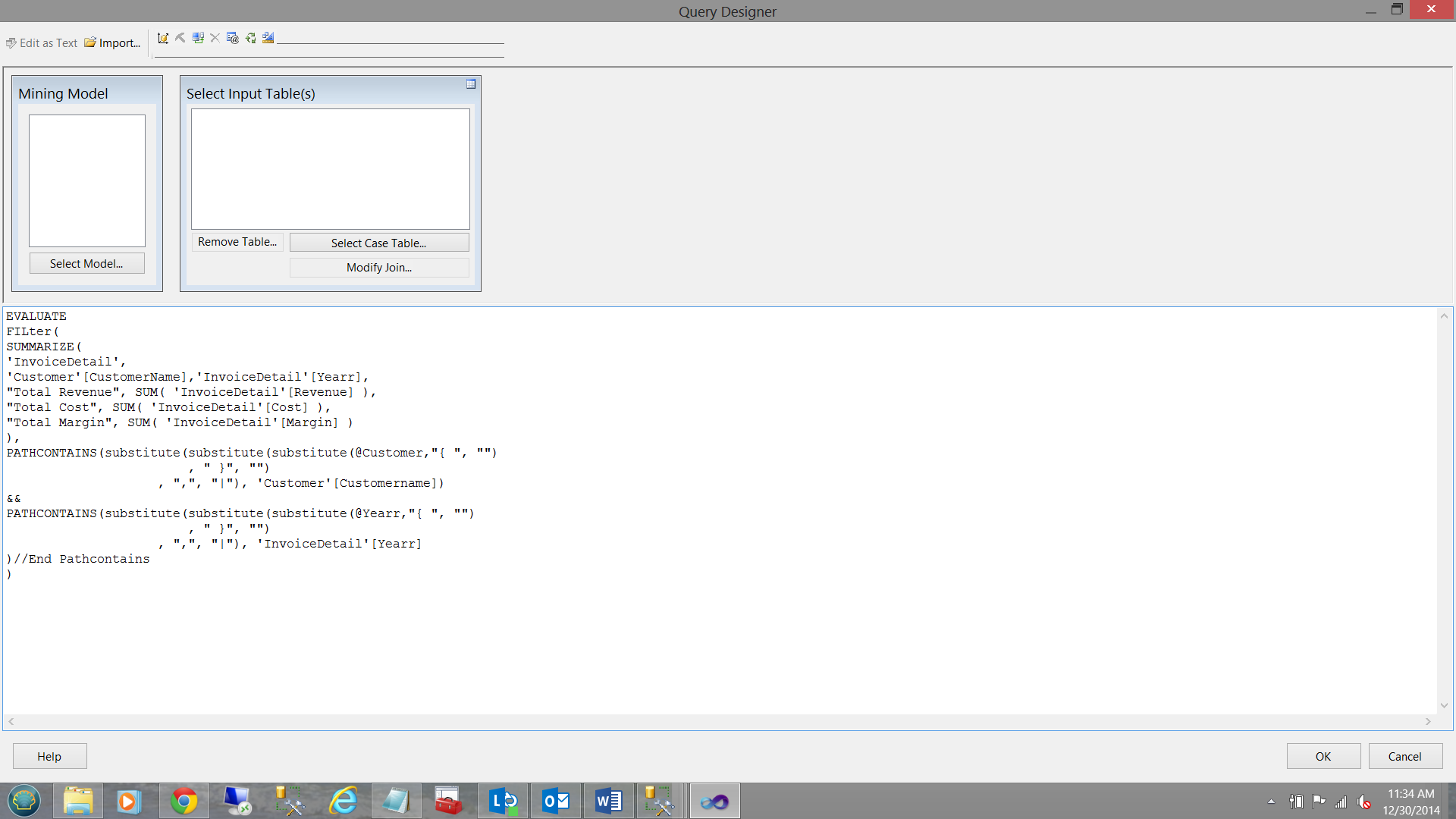
We place our DAX code into the box (see above). Click OK

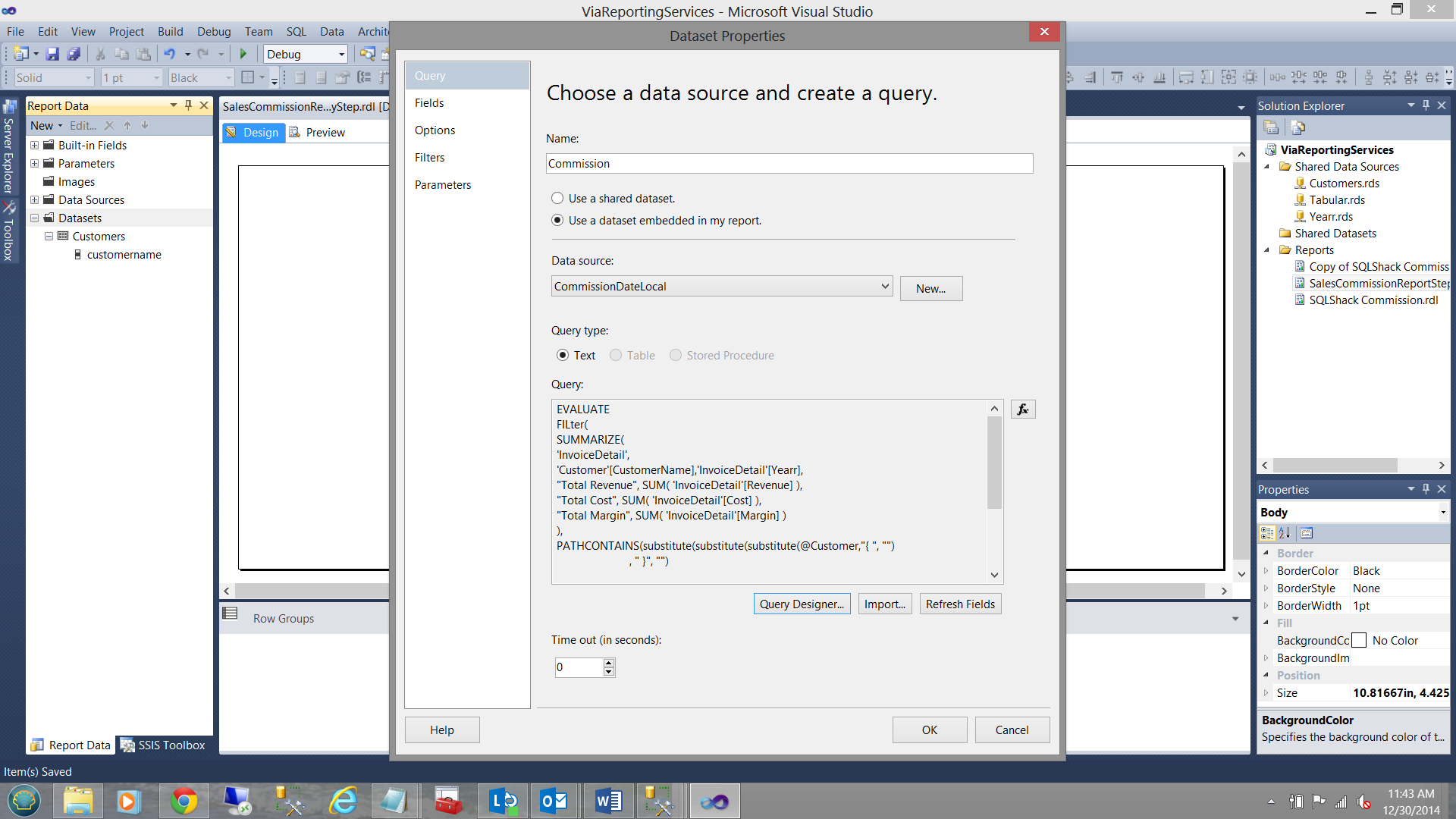
We find ourselves back at the “Dataset Properties” window.

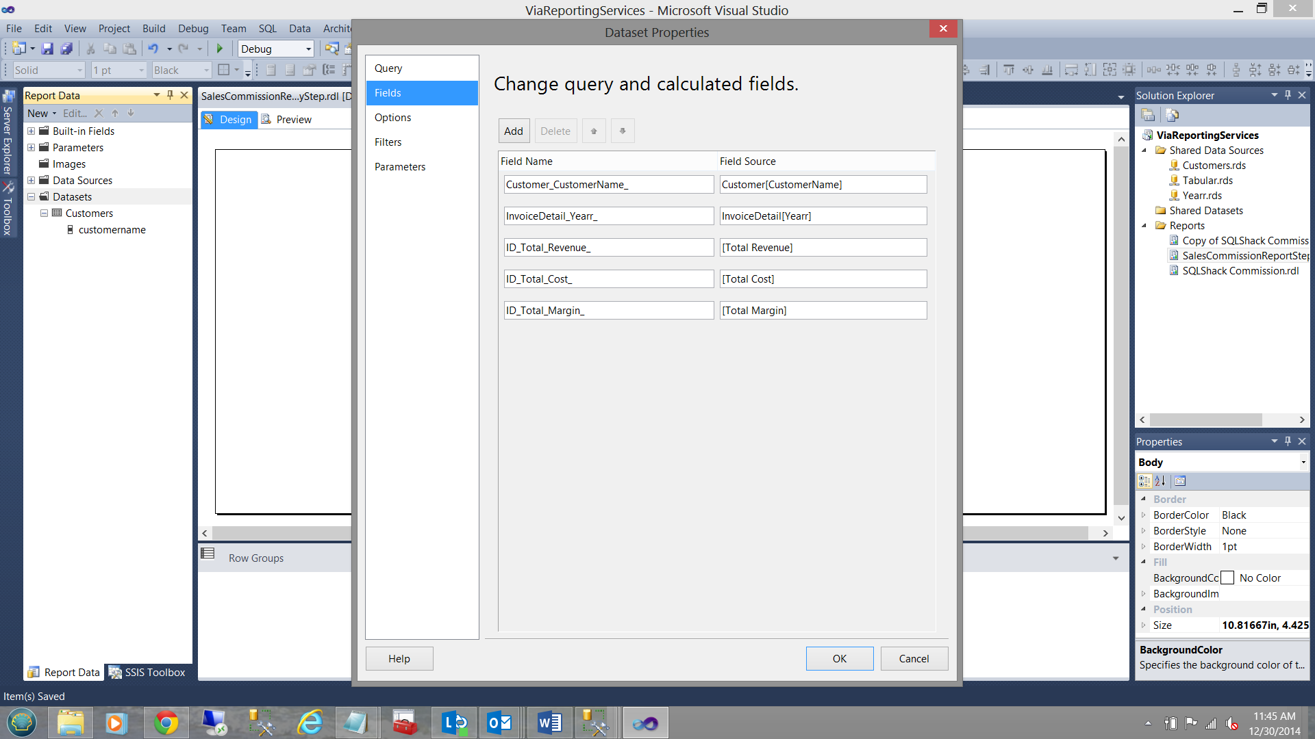
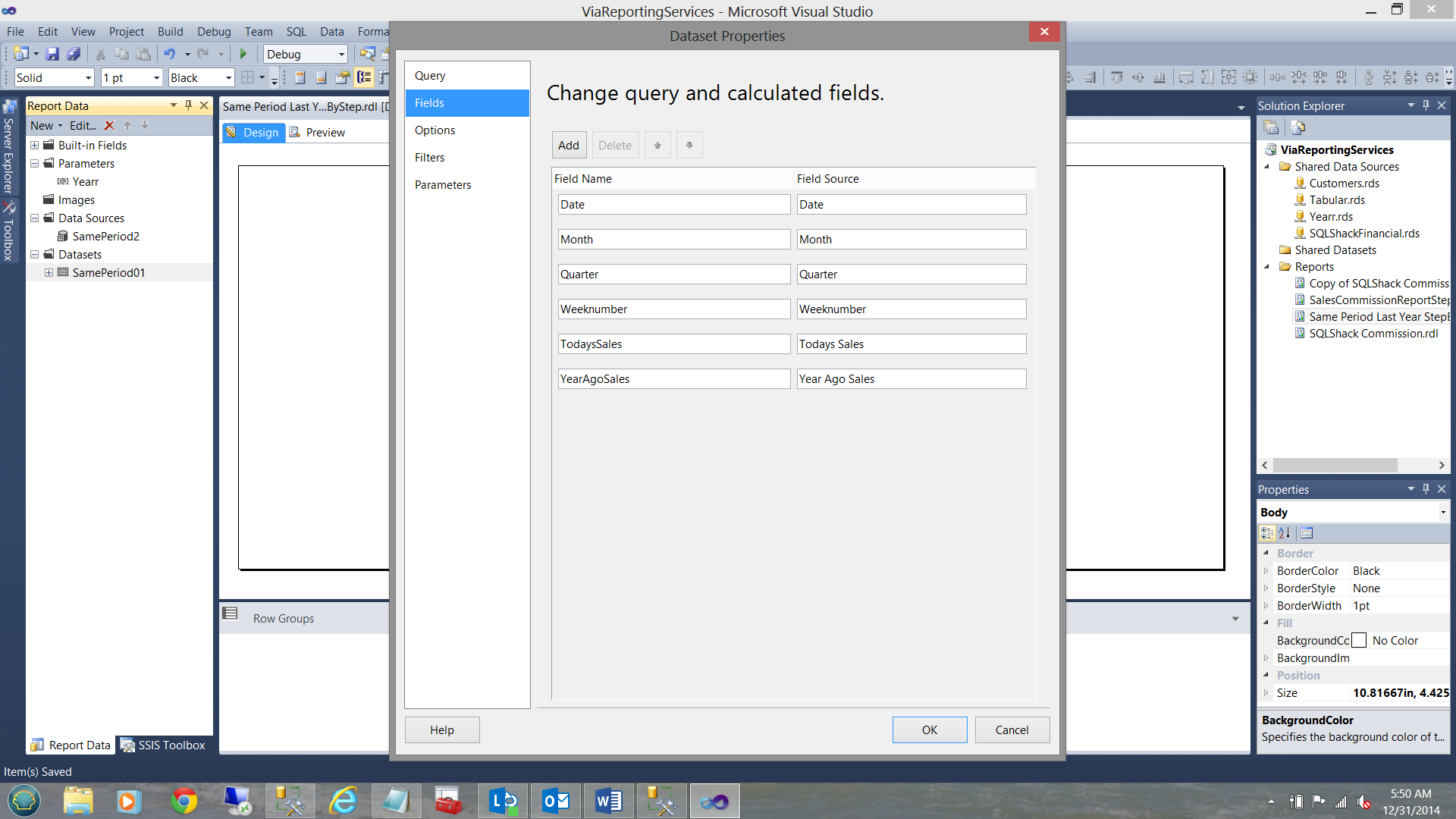
Clicking the “Fields” option (in the top left portion of the screen shot above) we see the fields that will be pulled.
We click “OK” to exit the “Dataset Properties” box.

Adding the eye candy!

Let us place a vertical bar chart onto the design surface (see below).
The astute reader will note that we have given the chart a title and placed the customer name on the X axis. Revenue is on the Y axis.

What is now required is to configure the chart.

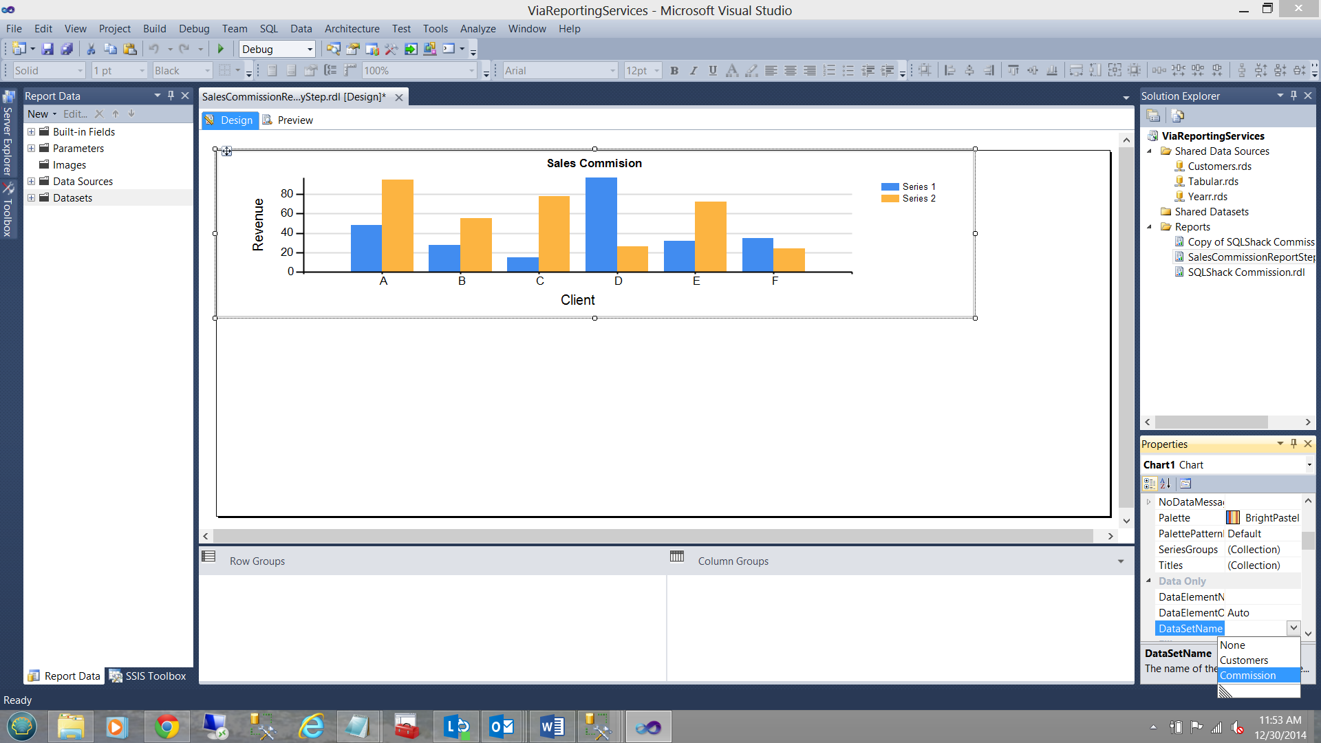
We set the data source for our chart to be the “Tabular” dataset Commission (see above bottom right).

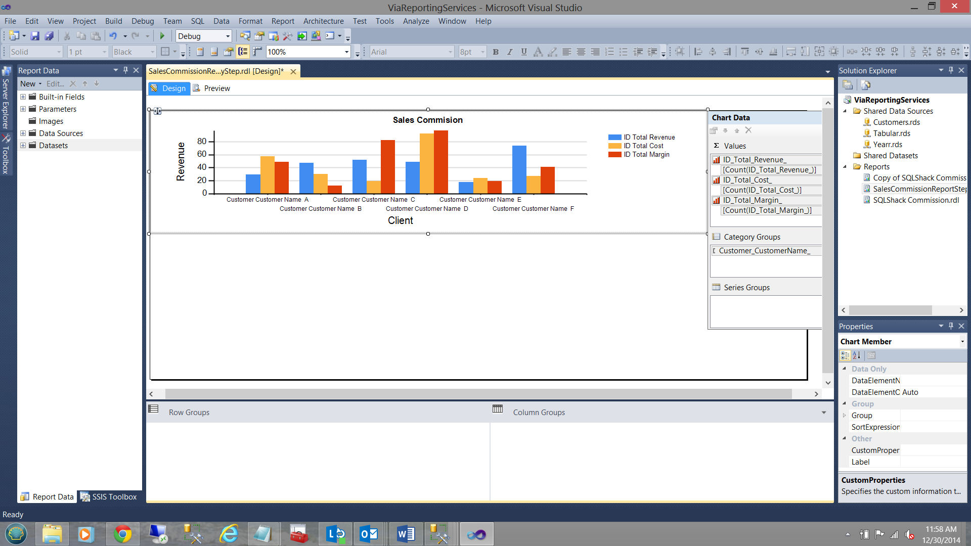
We set the ∑ values i.e. our measures (as seen above). Further, our “Category Groups” refer to our customers (see above).

Testing our report, we find the following when selecting customers.

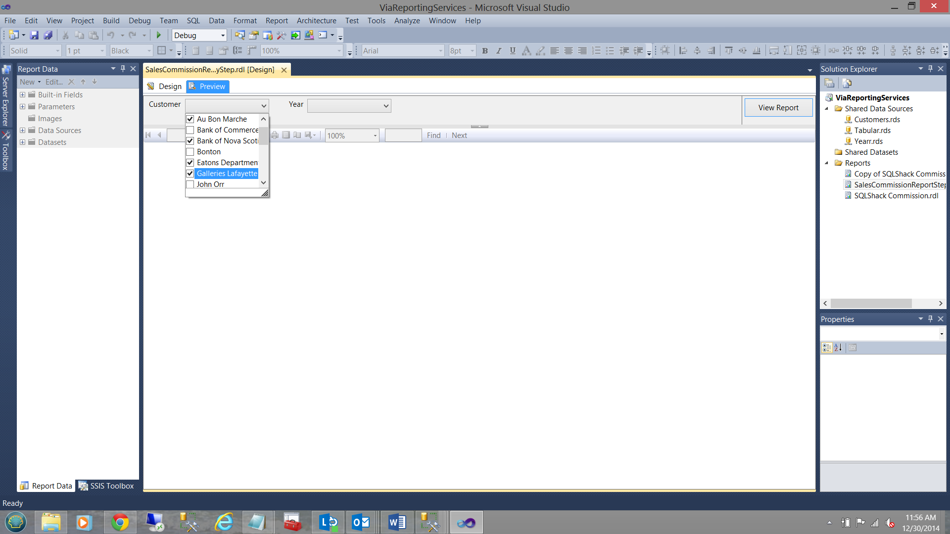
..and the following for years

The following result set is obtained (see below).

Adding the Matrix

SQLShack Industries management would also like to view the detailed results in a matrix format.
We now add a Matrix to our work surface and utilize the same “Commission” dataset.

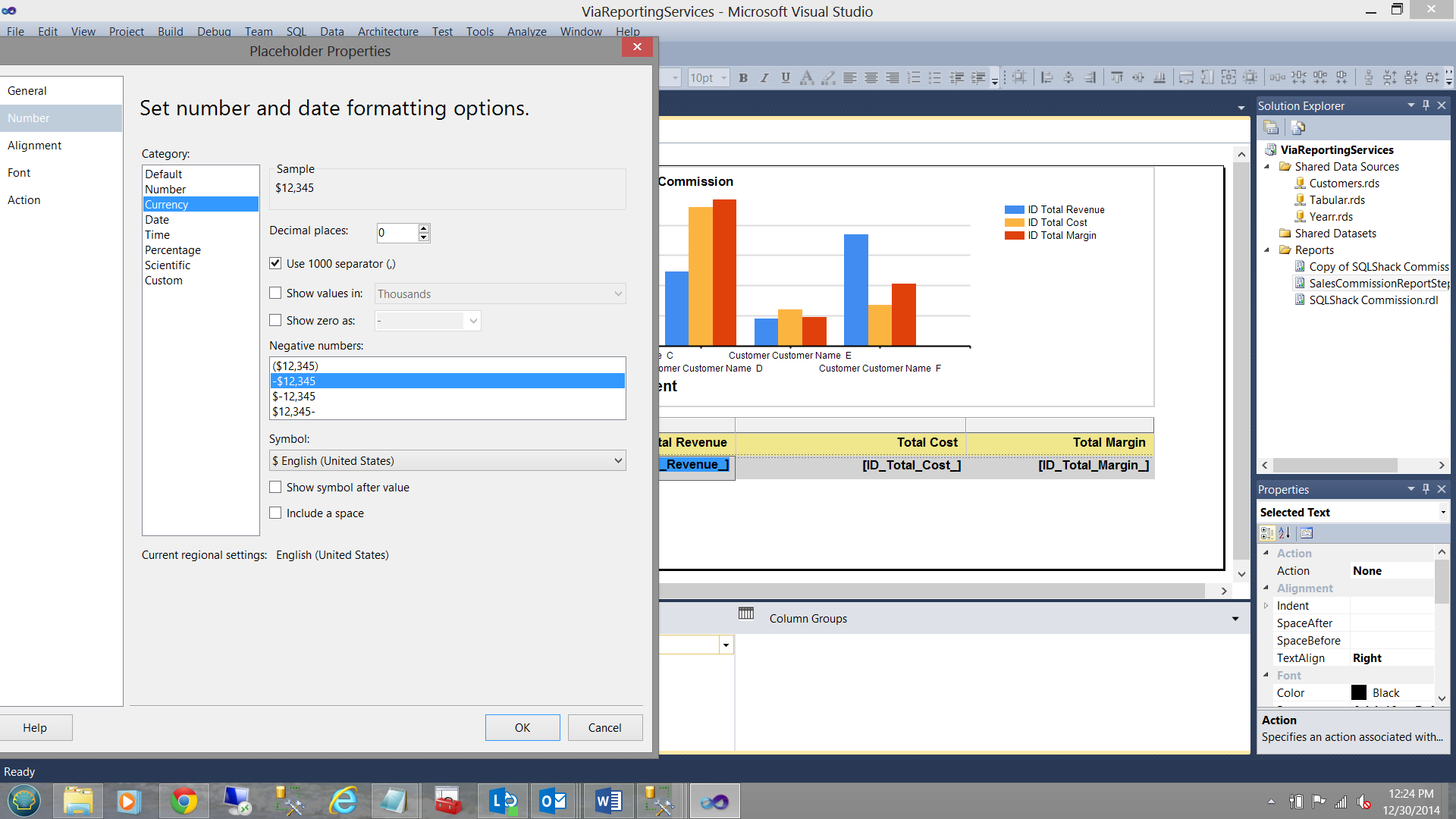
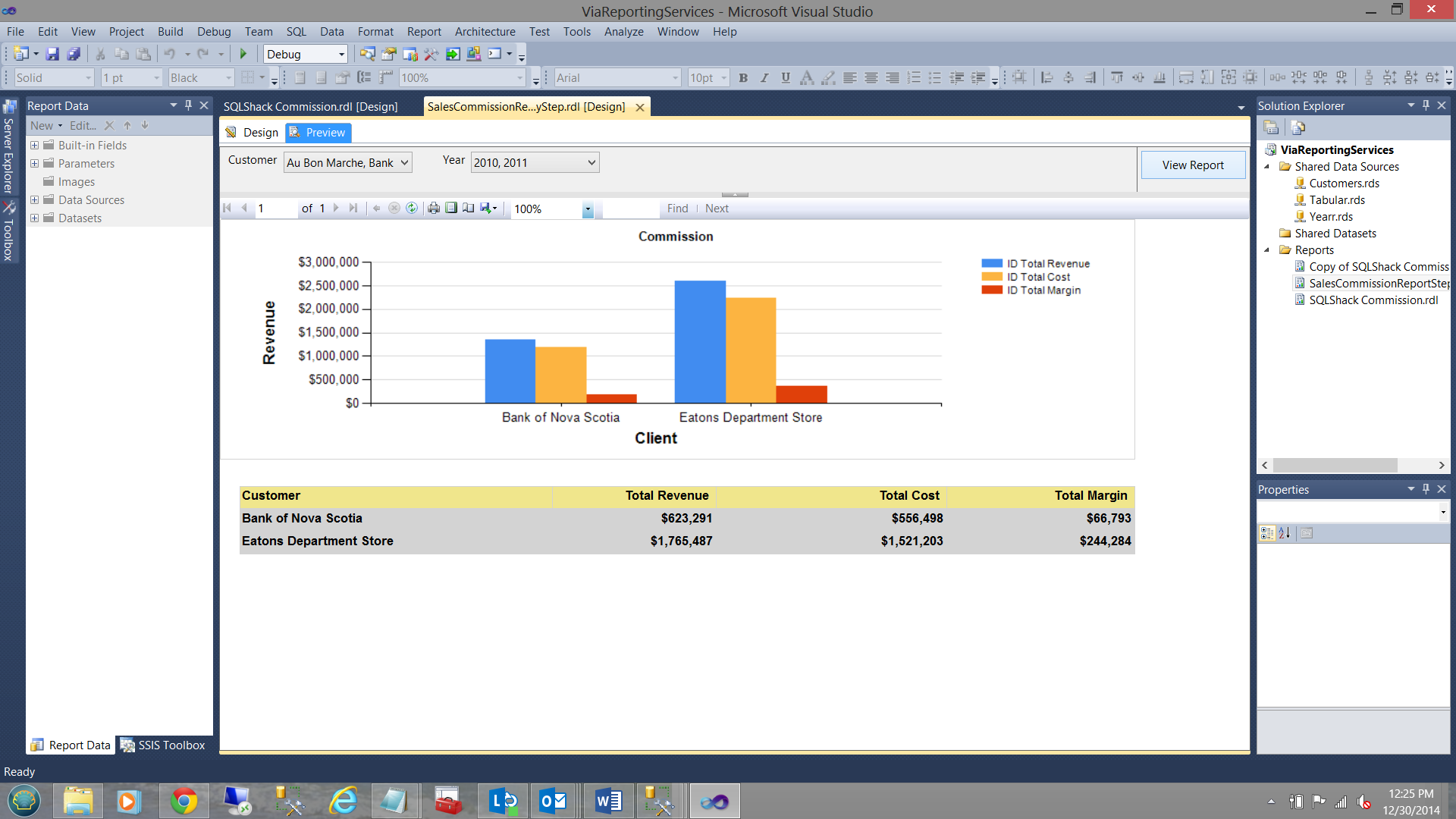
We format our fields and the end result may be seen below:

Now, having this report as a template

Not all DAX queries may be handled in this fashion. A case at hand.
SQLShack Industries would like to compare and contrast their daily sales to the same day of the prior year. This implies comparing the TOTAL SALES from December 31 2014 with sales from December 31, 2013.
Whilst a DAX query is totally in order, customer names are not really applicable as we are more interested in the daily sales aggregate.
For this challenge we are going to adopt a hybrid approach.
The primary data pull will be done utilizing DAX code. HOWEVER in this case we are going to utilize a bit of T-SQL as well.
Our plan of attack will be to create the DAX code, then create a LINKED SERVER to the Analysis Services Server and database and THEN through the use of an “Open Query” pull the data!!

Sound complicated!! Not really. Stay with me!

Our first task is to create a linked server to our Analysis Services database. The code to create this linked server may be seen below:

Setting up a linked server

From SSMS and THE DATABASE ENGINE

Now that we have created our linked server, we create our DAX query.
Once completed we must make one alteration to the code. FORTRAN and COBOL programmers will understand this perfectly. Every single quote MUST be replaced with quote quote.
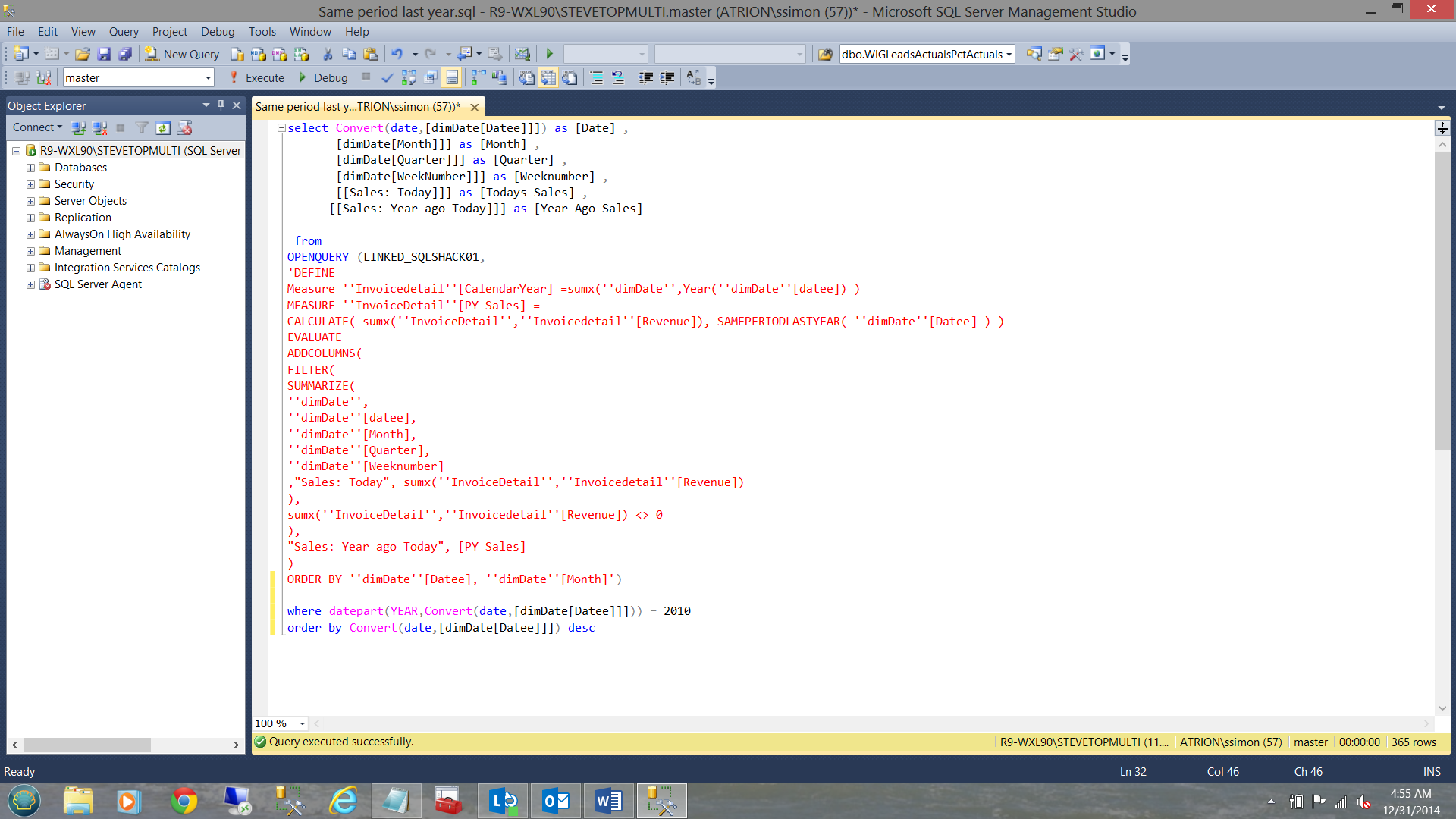
We must also add a single quote at the beginning of the query and one single quote at the end. The modified code for this query may be seen below:

Compiling all the pieces we now have our final query.

And the result set

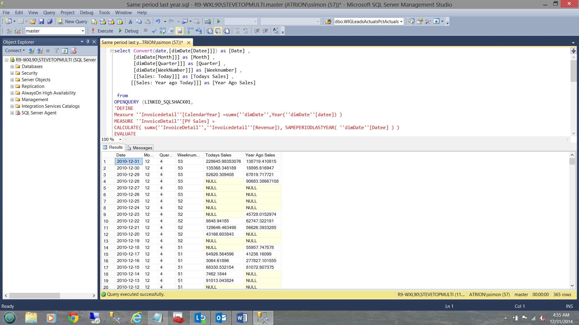
The assembled code for this query may be found below.

Our job is almost complete.

Remember that we want our query to extract only the data for one or more selected years. Further, Reporting Services will be passing a string containing the requested year(s) through to the stored procedure containing the code listings shown above.
As an example ‘2010, 2011, 2012’.

Fear not, dear reader, this is how we are going to handle this one.

1. The string will be passed into the stored procedure (as shown immediately above).
2. We shall split the string utilizing the code snippet below.
3. We shall then perform an inner join of the years from the split of the string with the year(s) from the dates within the query. The astute reader will ask: “INSTEAD OF AN INNER JOIN WHY NOT USE WHERE YEARR IN ()?” This is left to the reader to answer. Hint what happens should there be in excess of 1000 customers to the IN function?

The code for the string splitter

Let us now put all the pieces together and create our query!!!

Meanwhile back at the ranch!!

We have opened up SQL Server Data Tools (SSDT) and created a new report called ‘Same Period Last Year StepByStep’.
We begin by creating a new data source to connect with our SQLShackfinancial database where the stored procedure was created. It must be understood that the stored procedure could have be created in any database, as the data itself is originating from Analysis Services, via the linked server.

Having created the data source, we are now in a position to create the necessary dataset. By right clicking on the dataset folder (see above and left) we open the dataset properties box.

Once again we choose “Use a dataset embedded in my report” (see above).
We now create a new “local data source” (see below).

We click OK to leave this screen.
As our dataset will be populated via a stored procedure, we select this option (see below).

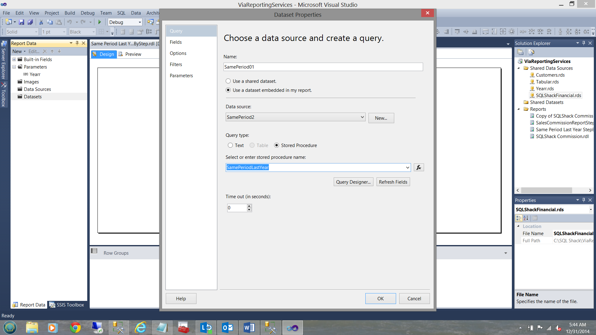
We now click “Refresh Fields” to see what we shall be pulling.

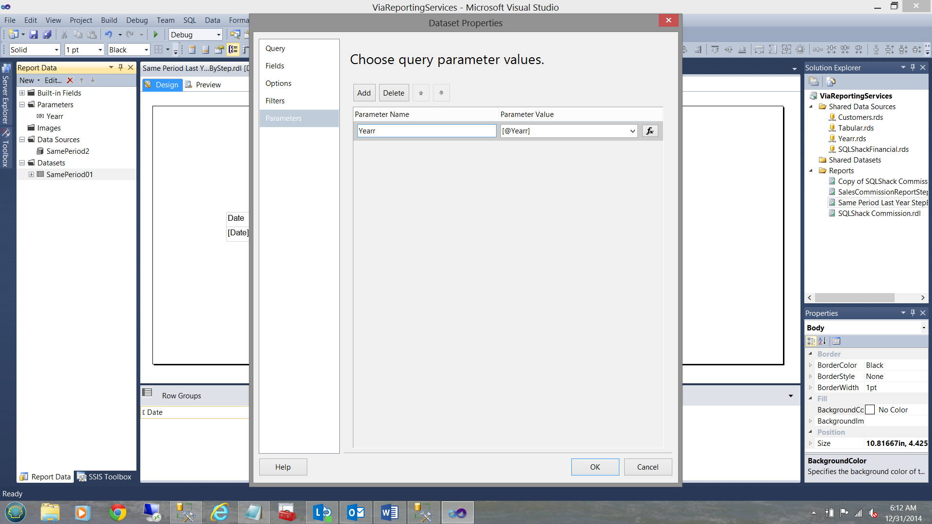
Finally we attach the “Yearr” parameter (above and left in the parameter folder) to the dataset (see below).

Moving on

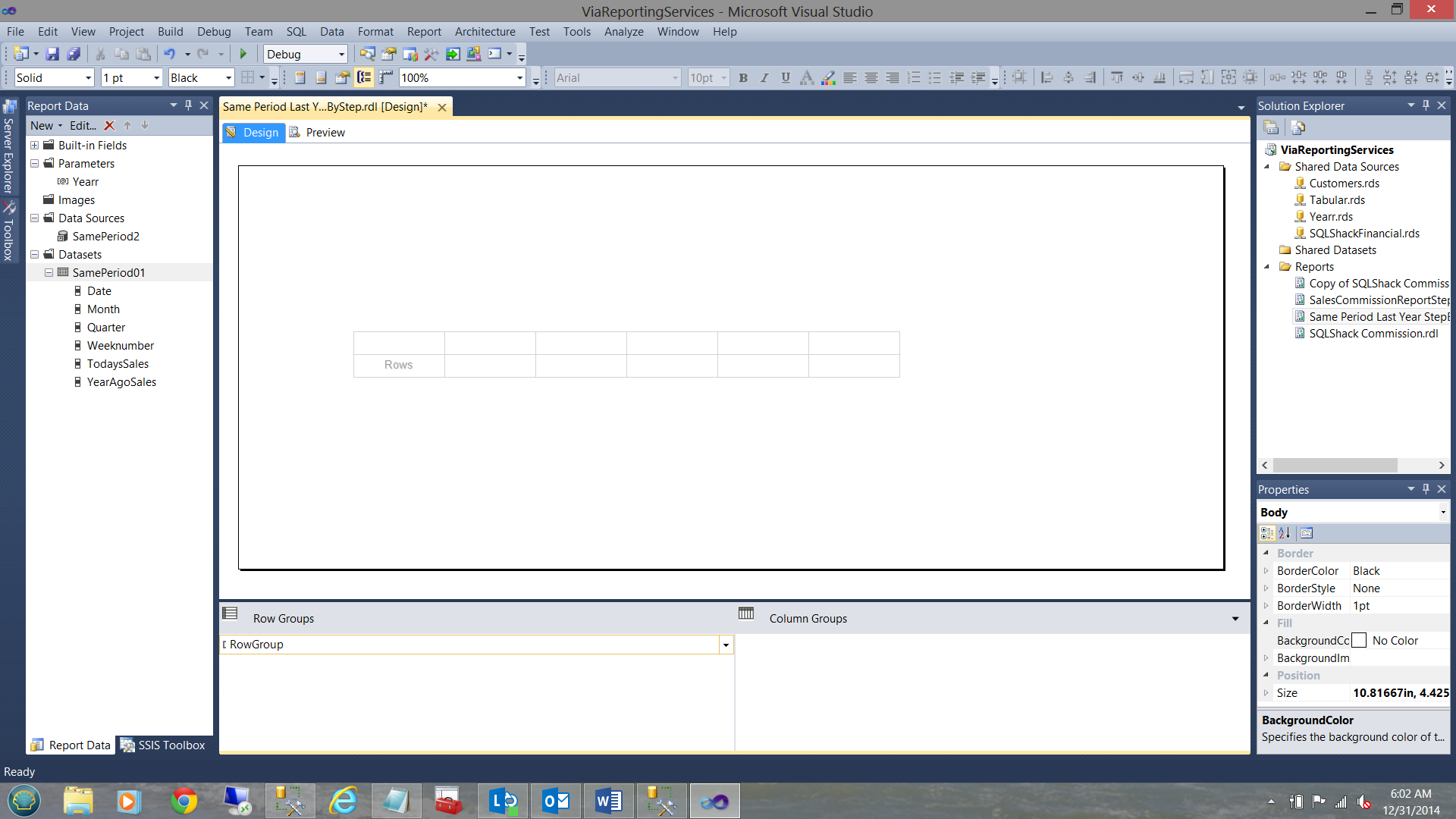
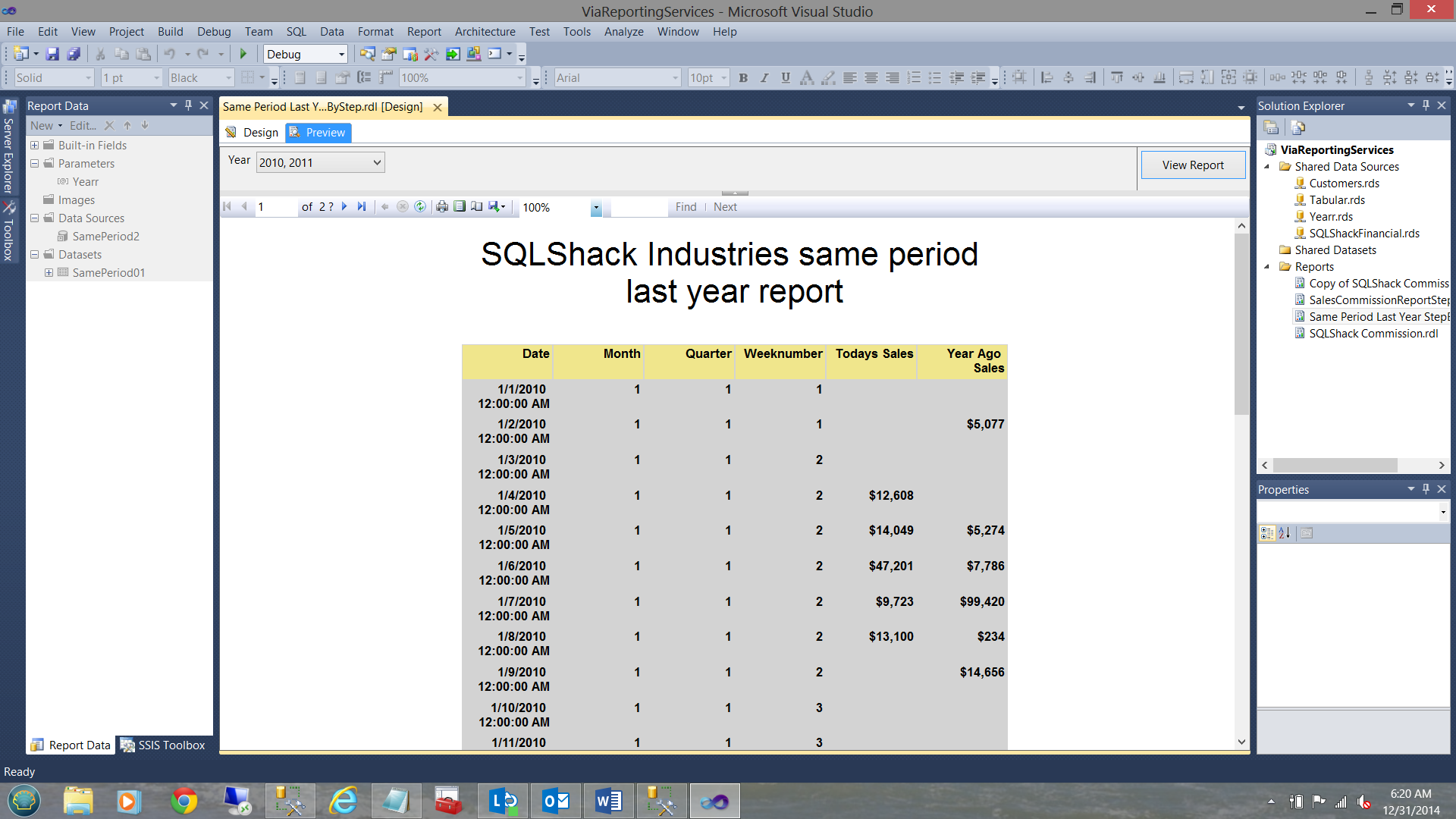
Placing a Matrix report item on the work surface and after having added a few more columns, we now see the following:

We must now attach the dataset (that we just created), to the Matrix(see below bottom right).

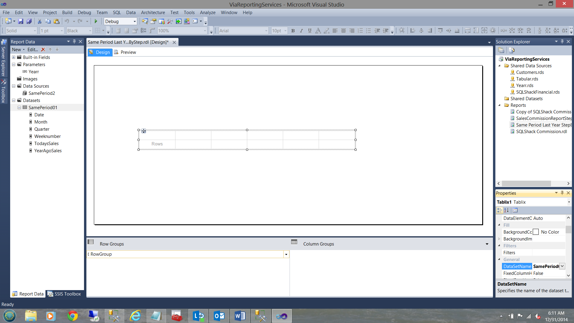
Having attached the dataset to the matrix, we now add the dataset fields to the matrix as may be seen below:

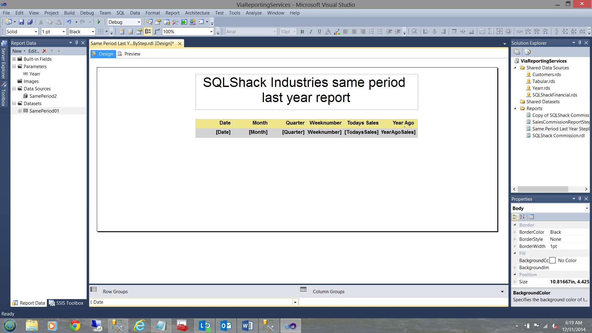
We are now DONE!!!

Let us now give it a whirl and see what we have!

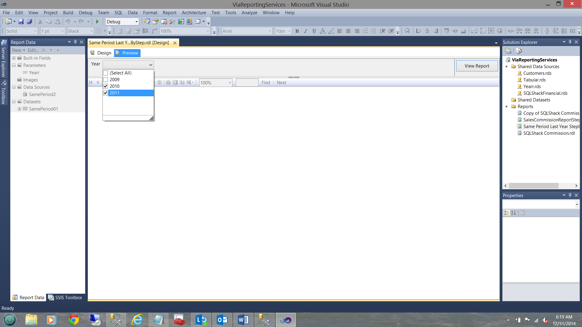
The results are:

Conclusions

Oft times we find ourselves in the position where we need to sharpen our tools and learn new techniques. When working with financial folks, a spreadsheet appearance appears to go over well. Further, the financial people seem to have an affinity to the working with a tabular model, based primarily on it look and feel.
Some reporting is very conducive to the tabular model. There are however strict rules that must be obeyed when utilizing DAX.
Other scenarios, like the “Same period last year” call for a hybrid approach.
Each scenario calls for distinct and innovative solutions.

The last word. My late Dad used to say, “What goes around, comes around”. You all have super skillsets. Do share your knowledge with others.

As always, happy programming and may this year be the best for you all.

• Author
• Recent Posts

Steve Simon

Steve Simon is a SQL Server MVP and a senior BI Development Engineer with Atrion Networking. He has been involved with database design and analysis for over 29 years.

Steve has presented papers at 8 PASS Summits and one at PASS Europe 2009 and 2010. He has recently presented a Master Data Services presentation at the PASS Amsterdam Rally.

Steve has presented 5 papers at the Information Builders' Summits. He is a PASS regional mentor.

View all posts by Steve Simon

Latest posts by Steve Simon (see all)

• Reporting in SQL Server – Using calculated Expressions within reports - December 19, 2016
• How to use Expressions within SQL Server Reporting Services to create efficient reports - December 9, 2016
• How to use SQL Server Data Quality Services to ensure the correct aggregation of data - November 9, 2016